Fitting MF (or other) datasets

12/09/22

For the basic (default) case, using AF data, see the basic demo notebook and PEMtk fitting setup & batch run demo notebook. This notebook is based on the latter, but demonstrates additionally:

Switching the fit dataset to use MF data as a function of polarization (as opposed to AF data as a function of alignment/time in the earlier demo case).
Switching the backend to calculate MFPADs (see the backends notebook for more).
Running fits.

Note that the methods here should be general, allowing for fitting of MF or AF/LF data vs. alignment, time, energy or polarization geometry depending on the dataset.

Setup

Here we’ll use the demo script, as per the PEMtk fitting setup & batch run demo notebook, then replace some of the defaults later. Alternatively, the MF case could be setup from scratch following the basic demo notebook.

[1]:

# Import & set paths
import pemtk
from pemtk.fit.fitClass import pemtkFit

from pathlib import Path

# Path for demo script
demoPath = Path(pemtk.__file__).parent.parent/Path('demos','fitting')

# Run demo script to configure workspace
%run {demoPath/"setup_fit_demo.py"}

*** ePSproc installation not found, setting for local copy.

* Setting plotter defaults with epsproc.basicPlotters.setPlotters(). Run directly to modify, or change options in local env.

* Set Holoviews with bokeh.

C:\Users\femtolab\.conda\envs\ePSdev\lib\site-packages\xyzpy\plot\xyz_cmaps.py:6: MatplotlibDeprecationWarning:
The revcmap function was deprecated in Matplotlib 3.2 and will be removed two minor releases later. Use Colormap.reversed() instead.
  return LinearSegmentedColormap(name, cm.revcmap(cmap._segmentdata))

*** Setting up demo fitting workspace and main `data` class object...
For more details see https://pemtk.readthedocs.io/en/latest/fitting/PEMtk_fitting_basic_demo_030621-full.html
To use local source code, pass the parent path to this script at run time, e.g. "setup_fit_demo ~/github"


* Loading packages...

* Set Holoviews with bokeh.

* Loading demo matrix element data from D:\code\github\ePSproc\data\photoionization\n2_multiorb...

*** Job subset details
Key: subset
No 'job' info set for self.data[subset].

*** Job orb6 details
Key: orb6
Dir D:\code\github\ePSproc\data\photoionization\n2_multiorb, 1 file(s).
{   'batch': 'ePS n2, batch n2_1pu_0.1-50.1eV, orbital A2',
    'event': ' N2 A-state (1piu-1)',
    'orbE': -17.096913836366,
    'orbLabel': '1piu-1'}

*** Job orb5 details
Key: orb5
Dir D:\code\github\ePSproc\data\photoionization\n2_multiorb, 1 file(s).
{   'batch': 'ePS n2, batch n2_3sg_0.1-50.1eV, orbital A2',
    'event': ' N2 X-state (3sg-1)',
    'orbE': -17.341816310545997,
    'orbLabel': '3sg-1'}


* Loading demo ADM data from D:\code\github\ePSproc\data\alignment\N2_ADM_VM_290816.mat...

* Subselecting data...
Subselected from dataset 'orb5', dataType 'matE': 36 from 11016 points (0.33%)
Subselected from dataset 'pol', dataType 'pol': 1 from 3 points (33.33%)
Subselected from dataset 'ADM', dataType 'ADM': 52 from 14764 points (0.35%)

* Calculating AF-BLMs...
Subselected from dataset 'sim', dataType 'AFBLM': 195 from 195 points (100.00%)

*Setting  up fit parameters (with constraints)...
Set 6 complex matrix elements to 12 fitting params, see self.params for details.

C:\Users\femtolab\.conda\envs\ePSdev\lib\site-packages\pandas\core\generic.py:3939: SettingWithCopyWarning:
A value is trying to be set on a copy of a slice from a DataFrame

See the caveats in the documentation: https://pandas.pydata.org/pandas-docs/stable/user_guide/indexing.html#returning-a-view-versus-a-copy
  self._update_inplace(obj)

Auto-setting parameters.

name	value	initial value	min	max	vary	expression
m_PU_SG_PU_1_n1_1_1	1.78461575	1.784615753610107	1.0000e-04	5.00000000	True
m_PU_SG_PU_1_1_n1_1	1.78461575	1.784615753610107	1.0000e-04	5.00000000	False	m_PU_SG_PU_1_n1_1_1
m_PU_SG_PU_3_n1_1_1	0.80290495	0.802904951323892	1.0000e-04	5.00000000	True
m_PU_SG_PU_3_1_n1_1	0.80290495	0.802904951323892	1.0000e-04	5.00000000	False	m_PU_SG_PU_3_n1_1_1
m_SU_SG_SU_1_0_0_1	2.68606212	2.686062120382649	1.0000e-04	5.00000000	True
m_SU_SG_SU_3_0_0_1	1.10915311	1.109153108617096	1.0000e-04	5.00000000	True
p_PU_SG_PU_1_n1_1_1	-0.86104140	-0.8610414024232179	-3.14159265	3.14159265	False
p_PU_SG_PU_1_1_n1_1	-0.86104140	-0.8610414024232179	-3.14159265	3.14159265	False	p_PU_SG_PU_1_n1_1_1
p_PU_SG_PU_3_n1_1_1	-3.12044446	-3.1204444620772467	-3.14159265	3.14159265	True
p_PU_SG_PU_3_1_n1_1	-3.12044446	-3.1204444620772467	-3.14159265	3.14159265	False	p_PU_SG_PU_3_n1_1_1
p_SU_SG_SU_1_0_0_1	2.61122920	2.611229196458127	-3.14159265	3.14159265	True
p_SU_SG_SU_3_0_0_1	-0.07867828	-0.07867827542158025	-3.14159265	3.14159265	True



*** Setup demo fitting workspace OK.

Set the (MF) data to fit

Here we’ll calculate some MF-\(\beta_{LM}\) parameters to use as the test data. Note this currently needs to be set as self.data['subset']['AFBLM'] for fitting (even if it’s a different datatype).

TODO: add dict key option here for different backends.

[5]:

# For MF case remove the existing AFBLM and update pols (these are set in demo script.)
# And for the polarisation geometries...
data.selOpts['pol'] = {}
data.setSubset(dataKey = 'pol', dataType = 'pol')

# Delete ADMs, since we don't
del(data.data['subset']['ADM'])

Subselected from dataset 'pol', dataType 'pol': 3 from 3 points (100.00%)

[6]:

# Set the backend function, see https://pemtk.readthedocs.io/en/latest/fitting/PEMtk_fitting_backends_demo_010922.html

# 21/08/22 - Change backend in dict
# data.fitOpts = {'backend':data.backends(backend='mfblmXprod')}
# 01/09/22 - Change to direct setting via self.backends
data.backends(backend='mfblmXprod')

[7]:

# Generate some data & update basis etc - now set by main fitting func.
# BLMtest, data.basis = data.afblmMatEfit(backend = ep.mfblmXprod, resetBasis = True)   # With backend by object
BLMtest, data.basis = data.afblmMatEfit(resetBasis = True)   # 21/08/22 With backend as set in data.fitOpts

data.setData('sim', BLMtest)  # Set simulated data to master structure as "sim"
data.setSubset('sim','AFBLM')   # Set to 'subset' to use for fitting.

Subselected from dataset 'sim', dataType 'AFBLM': 75 from 75 points (100.00%)

[8]:

# Show the data
data.data['subset']['AFBLM']

Note here there are 3 polarization geometries set, \((x,y,z)\), which is the default case. The MF backend generates only MF results (no alignment dependence). For a quick intro to the MF and AF/LF calculations, see the ePSproc intro notes.

[9]:

# Params should already be OK... (set by demo script)
data.params

[9]:

name	value	initial value	min	max	vary	expression
m_PU_SG_PU_1_n1_1_1	1.78461575	1.784615753610107	1.0000e-04	5.00000000	True
m_PU_SG_PU_1_1_n1_1	1.78461575	1.784615753610107	1.0000e-04	5.00000000	False	m_PU_SG_PU_1_n1_1_1
m_PU_SG_PU_3_n1_1_1	0.80290495	0.802904951323892	1.0000e-04	5.00000000	True
m_PU_SG_PU_3_1_n1_1	0.80290495	0.802904951323892	1.0000e-04	5.00000000	False	m_PU_SG_PU_3_n1_1_1
m_SU_SG_SU_1_0_0_1	2.68606212	2.686062120382649	1.0000e-04	5.00000000	True
m_SU_SG_SU_3_0_0_1	1.10915311	1.109153108617096	1.0000e-04	5.00000000	True
p_PU_SG_PU_1_n1_1_1	-0.86104140	-0.8610414024232179	-3.14159265	3.14159265	False
p_PU_SG_PU_1_1_n1_1	-0.86104140	-0.8610414024232179	-3.14159265	3.14159265	False	p_PU_SG_PU_1_n1_1_1
p_PU_SG_PU_3_n1_1_1	-3.12044446	-3.1204444620772467	-3.14159265	3.14159265	True
p_PU_SG_PU_3_1_n1_1	-3.12044446	-3.1204444620772467	-3.14159265	3.14159265	False	p_PU_SG_PU_3_n1_1_1
p_SU_SG_SU_1_0_0_1	2.61122920	2.611229196458127	-3.14159265	3.14159265	True
p_SU_SG_SU_3_0_0_1	-0.07867828	-0.07867827542158025	-3.14159265	3.14159265	True

Running a fit…

With the parameters and data set, everything is as per the previous demos - just call self.fit() to run a fit!

Statistics and outputs are handled by lmfit, which includes uncertainty estimates and correlations in the fitted parameters.

[10]:

# data.fit(fcn_kws = {'backend':ep.geomFunc.mfblmXprod})   # With backend by object
data.fit()   # 21/08/22 With backend as set in data.fitOpts

[11]:

data.data.keys()

[11]:

dict_keys(['subset', 'orb6', 'orb5', 'ADM', 'pol', 'sim', 0])

Note the new result appears in the main data dict by fit number, here 0.

[12]:

# Check fit outputs
fitInd = 0
data.data[fitInd]['results']

[12]:

Fit Statistics

fitting method	leastsq
# function evals	9
# data points	75
# variables	7
chi-square	3.3126e-31
reduced chi-square	4.8715e-33
Akaike info crit.	-5573.49196
Bayesian info crit.	-5557.26954

Variables

name	value	standard error	relative error	initial value	min	max	vary	expression
m_PU_SG_PU_1_n1_1_1	1.78461575	2.3867e-09	(0.00%)	1.784615753610107	1.0000e-04	5.00000000	True
m_PU_SG_PU_1_1_n1_1	1.78461575	2.3867e-09	(0.00%)	1.784615753610107	1.0000e-04	5.00000000	False	m_PU_SG_PU_1_n1_1_1
m_PU_SG_PU_3_n1_1_1	0.80290495	1.0738e-09	(0.00%)	0.802904951323892	1.0000e-04	5.00000000	True
m_PU_SG_PU_3_1_n1_1	0.80290495	1.0738e-09	(0.00%)	0.802904951323892	1.0000e-04	5.00000000	False	m_PU_SG_PU_3_n1_1_1
m_SU_SG_SU_1_0_0_1	2.68606212	1.7419e-09	(0.00%)	2.686062120382649	1.0000e-04	5.00000000	True
m_SU_SG_SU_3_0_0_1	1.10915311	7.1926e-10	(0.00%)	1.109153108617096	1.0000e-04	5.00000000	True
p_PU_SG_PU_1_n1_1_1	-0.86104140	0.00000000	(0.00%)	-0.8610414024232179	-3.14159265	3.14159265	False
p_PU_SG_PU_1_1_n1_1	-0.86104140	0.00000000	(0.00%)	-0.8610414024232179	-3.14159265	3.14159265	False	p_PU_SG_PU_1_n1_1_1
p_PU_SG_PU_3_n1_1_1	-3.12044446	1.0890e-16	(0.00%)	-3.1204444620772467	-3.14159265	3.14159265	True
p_PU_SG_PU_3_1_n1_1	-3.12044446	1.0890e-16	(0.00%)	-3.1204444620772467	-3.14159265	3.14159265	False	p_PU_SG_PU_3_n1_1_1
p_SU_SG_SU_1_0_0_1	2.61122920	8.1419e-10	(0.00%)	2.611229196458127	-3.14159265	3.14159265	True
p_SU_SG_SU_3_0_0_1	-0.07867828	8.1419e-10	(0.00%)	-0.07867827542158025	-3.14159265	3.14159265	True

Correlations (unreported correlations are < 0.100)

p_SU_SG_SU_1_0_0_1	p_SU_SG_SU_3_0_0_1	-1.0000
m_PU_SG_PU_1_n1_1_1	m_PU_SG_PU_3_n1_1_1	-1.0000
m_SU_SG_SU_1_0_0_1	m_SU_SG_SU_3_0_0_1	-1.0000
m_PU_SG_PU_3_n1_1_1	p_PU_SG_PU_3_n1_1_1	-0.5828
m_PU_SG_PU_1_n1_1_1	p_PU_SG_PU_3_n1_1_1	0.5828
m_SU_SG_SU_1_0_0_1	p_SU_SG_SU_1_0_0_1	0.2621
m_SU_SG_SU_1_0_0_1	p_SU_SG_SU_3_0_0_1	-0.2621
m_SU_SG_SU_3_0_0_1	p_SU_SG_SU_1_0_0_1	-0.2621
m_SU_SG_SU_3_0_0_1	p_SU_SG_SU_3_0_0_1	0.2621

For this case, with correct inputs, correct outputs are quickly returned.

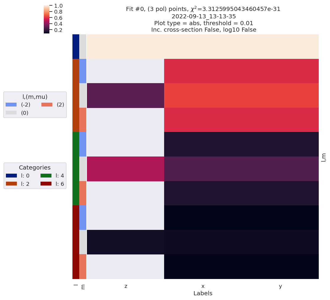
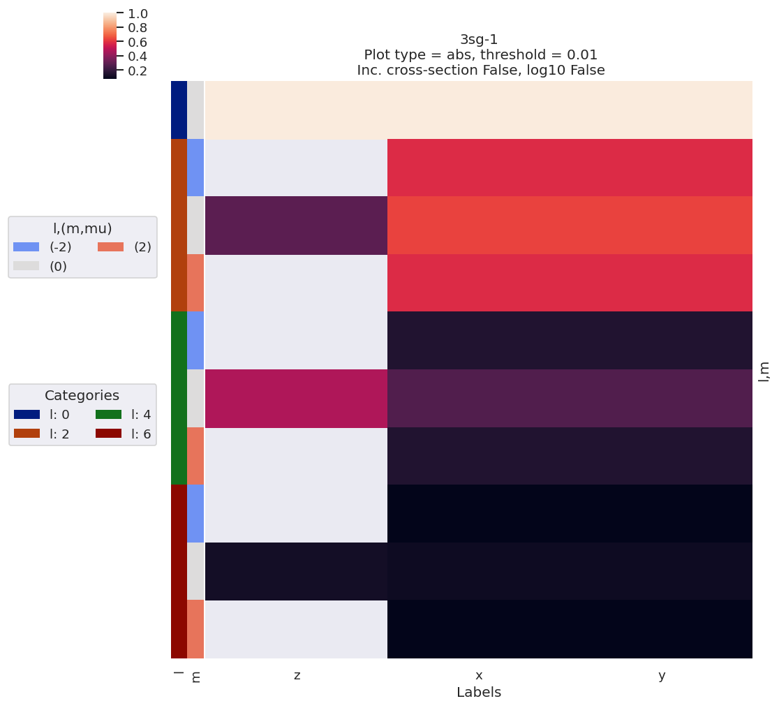
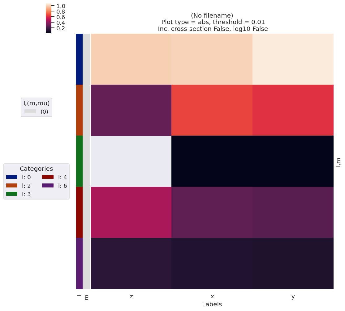
[13]:

# Quick plot with lmPlotFit - this defaults to the reference case plus the last fit
data.lmPlotFit(Etype='Labels')

Plotting data n2_3sg_0.1-50.1eV_A2.inp.out, pType=a, thres=0.01, with Seaborn
Plotting data (No filename), pType=a, thres=0.01, with Seaborn

../_images/fitting_PEMtk_fitting_demo_multi-fit_tests_130621-MFtests_120822-tidy-retest_20_1.png

../_images/fitting_PEMtk_fitting_demo_multi-fit_tests_130621-MFtests_120822-tidy-retest_20_2.png

Fit with randomized params…

The basic case above is a useful sanity check for the fitting routine. Now we can test from unknown (randomized) inputs to confirm that the fitting is actually useful…

[14]:

# Basic randomize routine, [0,1] interval for input parameter set
data.randomizeParams()

# data.fit(fcn_kws = {'backend':ep.geomFunc.mfblmXprod})   # With backend by object
data.fit()   # 21/08/22 With backend as set in data.fitOpts
data.lmPlotFit(Etype='Labels')

Plotting data n2_3sg_0.1-50.1eV_A2.inp.out, pType=a, thres=0.01, with Seaborn
Plotting data (No filename), pType=a, thres=0.01, with Seaborn

../_images/fitting_PEMtk_fitting_demo_multi-fit_tests_130621-MFtests_120822-tidy-retest_22_1.png

../_images/fitting_PEMtk_fitting_demo_multi-fit_tests_130621-MFtests_120822-tidy-retest_22_2.png

[15]:

# Check fit outputs
data.data[data.fitInd]['results']

[15]:

Fit Statistics

fitting method	leastsq
# function evals	83
# data points	75
# variables	7
chi-square	4.7958e-18
reduced chi-square	7.0526e-20
Akaike info crit.	-3300.72163
Bayesian info crit.	-3284.49921

Variables

name	value	standard error	relative error	initial value	min	max	vary	expression
m_PU_SG_PU_1_n1_1_1	0.08314518	4.9367e-07	(0.00%)	0.27981799849273714	1.0000e-04	5.00000000	True
m_PU_SG_PU_1_1_n1_1	0.08314518	0.00000000	(0.00%)	0.27981799849273714	1.0000e-04	5.00000000	False	m_PU_SG_PU_1_n1_1_1
m_PU_SG_PU_3_n1_1_1	0.03740731	2.2211e-07	(0.00%)	0.5537002130830051	1.0000e-04	5.00000000	True
m_PU_SG_PU_3_1_n1_1	0.03740731	0.00000000	(0.00%)	0.5537002130830051	1.0000e-04	5.00000000	False	m_PU_SG_PU_3_n1_1_1
m_SU_SG_SU_1_0_0_1	0.31810906	nan	(nan%)	0.6938920046815522	1.0000e-04	5.00000000	True
m_SU_SG_SU_3_0_0_1	0.13135648	nan	(nan%)	0.7601358965068807	1.0000e-04	5.00000000	True
p_PU_SG_PU_1_n1_1_1	-0.86104140	0.00000000	(0.00%)	-0.8610414024232179	-3.14159265	3.14159265	False
p_PU_SG_PU_1_1_n1_1	-0.86104140	0.00000000	(0.00%)	-0.8610414024232179	-3.14159265	3.14159265	False	p_PU_SG_PU_1_n1_1_1
p_PU_SG_PU_3_n1_1_1	1.39836166	4.9061e-10	(0.00%)	0.7549169336716605	-3.14159265	3.14159265	True
p_PU_SG_PU_3_1_n1_1	1.39836166	0.00000000	(0.00%)	0.7549169336716605	-3.14159265	3.14159265	False	p_PU_SG_PU_3_n1_1_1
p_SU_SG_SU_1_0_0_1	-3.08684154	nan	(nan%)	0.5995617123509013	-3.14159265	3.14159265	True
p_SU_SG_SU_3_0_0_1	-0.39693408	nan	(nan%)	0.8621457643783	-3.14159265	3.14159265	True

Correlations (unreported correlations are < 0.100)

m_PU_SG_PU_1_n1_1_1	m_PU_SG_PU_3_n1_1_1	1.0000
m_PU_SG_PU_3_n1_1_1	p_PU_SG_PU_3_n1_1_1	0.7263
m_PU_SG_PU_1_n1_1_1	p_PU_SG_PU_3_n1_1_1	0.7262

Note here that the \(\chi^2\) looks good, as do the MF-\(\beta_{LM}\), but the fitted parameters seem rather off from the reference case for the (m)agnitudes - this is because the input data was normalised by flux (i.e. \(\beta_{0,0}=1\)), so the fitting is only sensitive to relative magnitudes. The (p)hases, however, look good.

To get a better feel for this, run a batch of fits and look at the range of outputs more carefully…

Test batch run (multiple fits) with noisey data

Parallel run, see parallel execution for details.

In this test case, on an AMD Threadripper 2950X 16 core system, this took ~10 mins for 1000 fits.

[16]:

# Add noise with np.random.normal
# https://numpy.org/doc/stable/reference/random/generated/numpy.random.normal.html
# data.data['subset']['AFBLM']

import numpy as np
mu, sigma = 0, 0.05  # Up to approx 10% noise (+/- 0.05)
# creating a noise with the same dimension as the dataset (2,2)
noise = np.random.normal(mu, sigma, [data.data['subset']['AFBLM'].Labels.size, data.data['subset']['AFBLM'].l.size])
# data.BLMfitPlot()

# Set noise in Xarray & scale by l
import xarray as xr
noiseXR = xr.ones_like(data.data['subset']['AFBLM']) * noise
# data.data['subset']['AFBLM']['noise'] = ((data.data['subset']['AFBLM'].t, data.data['subset']['AFBLM'].l), noise)
# xr.where(noiseXR.l>0, noiseXR/noiseXR.l, noiseXR)
noiseXR = noiseXR.where(noiseXR.l<1, noiseXR/(noiseXR.l))  # Scale by L

data.data['subset']['AFBLM'] = data.data['subset']['AFBLM'] + noiseXR
data.data['subset']['AFBLM'] = data.data['subset']['AFBLM'].where(data.data['subset']['AFBLM'].m == 0, 0)

# data.BLMfitPlot(Etype='Labels', thres=None)

[17]:

data.lmPlotFit(keys='subset',Etype='Labels')

Set dataType (No dataType)
Plotting data (No filename), pType=a, thres=0.01, with Seaborn

../_images/fitting_PEMtk_fitting_demo_multi-fit_tests_130621-MFtests_120822-tidy-retest_27_1.png

[18]:

data.multiFit(nRange = [0,1000])

100%|##############################################################################| 1000/1000 [13:33<00:00,  1.23it/s]

[19]:

# Data IO with self.writeFitData()
# This will default to the working dir and set a data-stamped file name if nothing is passed.
data.writeFitData(outStem='dataDump_100fitTests_MFBLM_multiFit_noise-3')
# data.writeFitData()

# Runs
# 1. dataDump_100fitTests_MFBLM_multiFit_noise-3_130922_10-42-09.pickle
# 2. dataDump_100fitTests_MFBLM_multiFit_noise-3_130922_13-27-15.pickle

[19]:

WindowsPath('D:/code/python/jupyterNotebooks/dev/PEMtk/fitting/MF_fit_dev_120822/dataDump_100fitTests_MFBLM_multiFit_noise-3_130922_13-27-15.pickle')

Data overview

For more on the data structures used here, see the setup & batch runs notebook.

For more on the analysis routines, see the fit fidelity and analysis routines notebooks.

[20]:

# Load data if required
# import pickle
# with open('dataDump_1000fitTests_MFBLM_multiFit_noise-1_220822.pickle', 'wb') as handle:
#     pickle.dump(data.data, handle, protocol=pickle.HIGHEST_PROTOCOL)

# data.loadFitData('dataDump_1000fitTests_MFBLM_multiFit_noise-1_220822.pickle')

# data.loadFitData('dataDump_100fitTests_MFBLM_multiFit_noise-2_120922_19-34-54.pickle')

[21]:

# Run basic stats
# TODO: add more outputs here & tidy up output formatting.
data.analyseFits(keyDims='Labels')

*** Warning: found MultiIndex for DataFrame data.index - checkDims may have issues with Pandas MultiIndex, but will try anyway.
*** Warning: found MultiIndex for DataFrame data.index - checkDims may have issues with Pandas MultiIndex, but will try anyway.

[22]:

data.fitsSummary

[22]:

{'Fits': 999,
 'Success': 999,
 'Minima': {'chisqr': 1.34668471213695, 'redchi': 0.019804186943190444},
 'Stats': {'chisqr': min       1.346685
  mean      1.359765
  median    1.346685
  max       2.961047
  std       0.074494
  var       0.005549
  Name: chisqr, dtype: float64,
  'redchi': min       0.019804
  mean      0.019997
  median    0.019804
  max       0.043545
  std       0.001096
  var       0.000001
  Name: redchi, dtype: float64}}

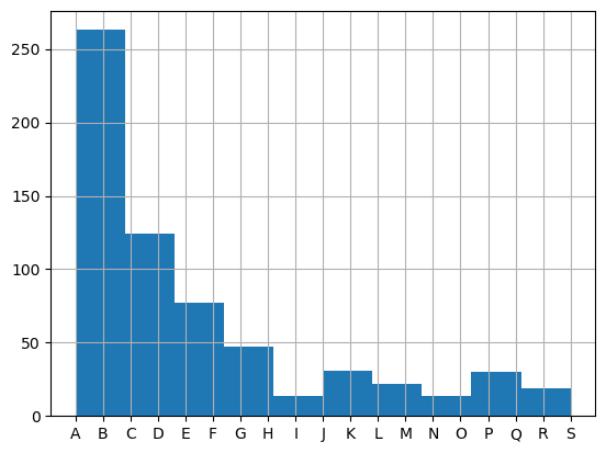
[23]:

# Basic histogram of fit sets
# Note this defaults to Holoviews/Bokeh for plotting, which produces an interactive plot.
# Set backend = 'mpl' if Holoviews is not available.
data.fitHist(bins = 100)

[39]:

# Try zooming in on the good results - note in this example case the spread is small!

# data.fitHist(thres = 0.01992, bins = 100)  # With threshold

# binRange = [0.0199115479, 0.0199115481]
# binRange = [0.01980418694, 0.019804187]
# binRange = [data.fitsSummary['Minima']['redchi'], data.fitsSummary['Minima']['redchi'] + data.fitsSummary['Minima']['redchi']*1e-8]

# Rough guess from variance?
binRange = [data.fitsSummary['Minima']['redchi'], data.fitsSummary['Minima']['redchi'] + data.fitsSummary['Stats']['redchi']['var']*1e-5]

data.fitHist(binRange = binRange, bins = 100, thres=binRange[1])  # With bins set, NOTE thres=binRange[1] sets X-lims here, now fixed in fitHist()

Mask selected 524 results (from 999).

[51]:

# Classify...
# data.classifyFits(bins = [0.01991154792, 0.019911548,20])
# data.classifyFits(bins = [0.01991154792, 0.01991154793,20])   # Slice best fit region
data.classifyFits(bins = [0.019804186942, 0.01980418697,20])   # Slice best fit region
# data.classifyFits(bins = [*binRange, 20])

	success				chisqr				redchi
	count	unique	top	freq	count	unique	top	freq	count	unique	top	freq
redchiGroup
A	42	1	True	42	42.0	42.0	1.346685	1.0	42.0	42.0	0.019804	1.0
B	221	1	True	221	221.0	221.0	1.346685	1.0	221.0	221.0	0.019804	1.0
C	76	1	True	76	76.0	76.0	1.346685	1.0	76.0	76.0	0.019804	1.0
D	48	1	True	48	48.0	48.0	1.346685	1.0	48.0	48.0	0.019804	1.0
E	53	1	True	53	53.0	53.0	1.346685	1.0	53.0	53.0	0.019804	1.0
F	24	1	True	24	24.0	24.0	1.346685	1.0	24.0	24.0	0.019804	1.0
G	18	1	True	18	18.0	18.0	1.346685	1.0	18.0	18.0	0.019804	1.0
H	29	1	True	29	29.0	29.0	1.346685	1.0	29.0	29.0	0.019804	1.0
I	14	1	True	14	14.0	14.0	1.346685	1.0	14.0	14.0	0.019804	1.0
J	13	1	True	13	13.0	13.0	1.346685	1.0	13.0	13.0	0.019804	1.0
K	18	1	True	18	18.0	18.0	1.346685	1.0	18.0	18.0	0.019804	1.0
L	14	1	True	14	14.0	14.0	1.346685	1.0	14.0	14.0	0.019804	1.0
M	8	1	True	8	8.0	8.0	1.346685	1.0	8.0	8.0	0.019804	1.0
N	10	1	True	10	10.0	10.0	1.346685	1.0	10.0	10.0	0.019804	1.0
O	4	1	True	4	4.0	4.0	1.346685	1.0	4.0	4.0	0.019804	1.0
P	18	1	True	18	18.0	18.0	1.346685	1.0	18.0	18.0	0.019804	1.0
Q	12	1	True	12	12.0	12.0	1.346685	1.0	12.0	12.0	0.019804	1.0
R	10	1	True	10	10.0	10.0	1.346685	1.0	10.0	10.0	0.019804	1.0
S	9	1	True	9	9.0	9.0	1.346685	1.0	9.0	9.0	0.019804	1.0

*** Warning: found MultiIndex for DataFrame data.index - checkDims may have issues with Pandas MultiIndex, but will try anyway.
*** Warning: found MultiIndex for DataFrame data.index - checkDims may have issues with Pandas MultiIndex, but will try anyway.

../_images/fitting_PEMtk_fitting_demo_multi-fit_tests_130621-MFtests_120822-tidy-retest_36_2.png

Examine trial parameter sets

[52]:

# Correct magnitudes (renorm) and phases (to ref)
data.phaseCorrection()

*** Warning: found MultiIndex for DataFrame data.index - checkDims may have issues with Pandas MultiIndex, but will try anyway.
*** Warning: found MultiIndex for DataFrame data.index - checkDims may have issues with Pandas MultiIndex, but will try anyway.
Set ref param = PU_SG_PU_1_1_n1_1

		Param	PU_SG_PU_1_1_n1_1	PU_SG_PU_1_n1_1_1	PU_SG_PU_3_1_n1_1	PU_SG_PU_3_n1_1_1	SU_SG_SU_1_0_0_1	SU_SG_SU_3_0_0_1
Fit	Type	redchiGroup
0	m	E	1.771928	1.771928	0.830945	0.830945	4.986125	2.161857
	n	E	0.290537	0.290537	0.136247	0.136247	0.817557	0.354472
	p	E	-0.861041	-0.861041	1.018645	1.018645	0.777926	-2.888186
	pc	E	-0.861041	-0.861041	1.018645	1.018645	0.777926	-2.888186
2	m	B	4.695653	4.695653	2.201952	2.201952	4.956811	2.149144
...	...	...	...	...	...	...	...	...
996	pc	B	-0.861041	-0.861041	-2.740728	-2.740728	-2.176238	0.440835
998	m	I	1.562246	1.562246	0.732626	0.732626	4.296351	1.862785
	n	I	0.295854	0.295854	0.138743	0.138743	0.813631	0.352769
	p	I	-0.861041	-0.861041	-2.740727	-2.740727	3.123349	-0.542763
	pc	I	-0.861041	-0.861041	-2.740727	-2.740727	3.123349	-0.542763

2564 rows × 6 columns

[53]:

# Test best group, normalized magnitudes
plotGroup = 'A'
data.paramPlot(selectors={'Type':'n', 'redchiGroup':plotGroup}, hue = 'redchi', backend='hv', hvType='violin', remap = 'lmMap', hRound = 30)  # New form with dict

*** Warning: found MultiIndex for DataFrame data.index - checkDims may have issues with Pandas MultiIndex, but will try anyway.

[54]:

# Test best group, corrected phases
data.paramPlot(selectors={'Type':'pc', 'redchiGroup':plotGroup}, hue = 'redchi', backend='hv', hvType='violin', remap = 'lmMap', hRound = 30)  # New form with dict

*** Warning: found MultiIndex for DataFrame data.index - checkDims may have issues with Pandas MultiIndex, but will try anyway.

Based on these plots, in this case we can conclude:

There is some spread in the retrieved normalised magnitudes, but there are preferred regions of solution space, although the m=0 paramters are less well defined.
The sign of the phases was also undefined in this case (this is in line with the AF reconstruction procedure).
The relative phase between the \(\sigma_u\) continuum (m=0), and the \(\pi_u\) continuum is undefined in this case, which is due to a lack of cross-terms between continua in this case.

Overall, it seems like there is the expected level of convergence, and that the matrix elements were constrained as expect, with only relative magnitudes and phases obtained (per continuum) in this manner.

The values can be inspected a little more carefully by forcing the phases to abs values (i.e. \(0:\pi\) range), and comparing the normalized and phase-corrected values with the known inputs…

[55]:

data.phaseCorrection(absFlag=True, useRef = False)  # Recompute phase corrections without reference shift & using 0:pi only
data.paramPlot(selectors={'Type':'pc', 'redchiGroup':plotGroup}, hue = 'redchi', backend='hv', hvType='violin', remap = 'lmMap', hRound = 30)  # New form with dict

*** Warning: found MultiIndex for DataFrame data.index - checkDims may have issues with Pandas MultiIndex, but will try anyway.
*** Warning: found MultiIndex for DataFrame data.index - checkDims may have issues with Pandas MultiIndex, but will try anyway.
Set ref param = PU_SG_PU_1_1_n1_1

		Param	PU_SG_PU_1_1_n1_1	PU_SG_PU_1_n1_1_1	PU_SG_PU_3_1_n1_1	PU_SG_PU_3_n1_1_1	SU_SG_SU_1_0_0_1	SU_SG_SU_3_0_0_1
Fit	Type	redchiGroup
0	m	E	1.771928	1.771928	0.830945	0.830945	4.986125	2.161857
	n	E	0.290537	0.290537	0.136247	0.136247	0.817557	0.354472
	p	E	-0.861041	-0.861041	1.018645	1.018645	0.777926	-2.888186
	pc	E	0.000000	0.000000	1.879686	1.879686	1.638968	2.027144
2	m	B	4.695653	4.695653	2.201952	2.201952	4.956811	2.149144
...	...	...	...	...	...	...	...	...
996	pc	B	0.000000	0.000000	1.879686	1.879686	1.315196	1.301877
998	m	I	1.562246	1.562246	0.732626	0.732626	4.296351	1.862785
	n	I	0.295854	0.295854	0.138743	0.138743	0.813631	0.352769
	p	I	-0.861041	-0.861041	-2.740727	-2.740727	3.123349	-0.542763
	pc	I	0.000000	0.000000	1.879686	1.879686	2.298795	0.318278

2564 rows × 6 columns

*** Warning: found MultiIndex for DataFrame data.index - checkDims may have issues with Pandas MultiIndex, but will try anyway.

[56]:

# Get parameter statistics & compare with ref

# Specify subselection criteria with a dictionary of selectors (currently uses index values only) & report
data.paramsReport(inds = {'redchiGroup':plotGroup})
data.paramsCompare()

# Final comparison with formatting
import pandas as pd
# pd.options.display.precision = 5
pd.options.display.float_format = '{:.4f}'.format
data.paramsSummaryComp

*** Warning: found MultiIndex for DataFrame data.index - checkDims may have issues with Pandas MultiIndex, but will try anyway.
*** Warning: found MultiIndex for DataFrame data.index - checkDims may have issues with Pandas MultiIndex, but will try anyway.
*** Warning: found MultiIndex for DataFrame data.index - checkDims may have issues with Pandas MultiIndex, but will try anyway.
Set ref param = PU_SG_PU_1_1_n1_1

	Param	PU_SG_PU_1_1_n1_1	PU_SG_PU_1_n1_1_1	PU_SG_PU_3_1_n1_1	PU_SG_PU_3_n1_1_1	SU_SG_SU_1_0_0_1	SU_SG_SU_3_0_0_1
Fit	Type
ref	m	0.279818	0.279818	0.553700	0.553700	0.693892	0.760136
	n	0.206901	0.206901	0.409412	0.409412	0.513072	0.562053
	p	-0.861041	-0.861041	0.754917	0.754917	0.599562	0.862146
	pc	0.000000	0.000000	1.615958	1.615958	1.460603	1.723187

C:\Users\femtolab\.conda\envs\ePSdev\lib\site-packages\IPython\core\interactiveshell.py:2886: PerformanceWarning: indexing past lexsort depth may impact performance.
  return runner(coro)

[56]:

		Param	PU_SG_PU_1_1_n1_1	PU_SG_PU_1_n1_1_1	PU_SG_PU_3_1_n1_1	PU_SG_PU_3_n1_1_1	SU_SG_SU_1_0_0_1	SU_SG_SU_3_0_0_1
Type	Source	dType
m	mean	num	2.9271	2.9271	1.3726	1.3726	2.4727	1.0721
	ref	num	0.2798	0.2798	0.5537	0.5537	0.6939	0.7601
	diff	%	90.4405	90.4405	59.6610	59.6610	71.9377	29.0978
	diff	num	2.6473	2.6473	0.8189	0.8189	1.7788	0.3120
	std	%	60.7753	60.7753	60.7753	60.7753	78.9698	78.9698
	std	num	1.7790	1.7790	0.8342	0.8342	1.9527	0.8466
	diff/std	%	148.8113	148.8113	98.1664	98.1664	91.0952	36.8467
n	mean	num	0.4920	0.4920	0.2307	0.2307	0.4436	0.1924
	ref	num	0.2069	0.2069	0.4094	0.4094	0.5131	0.5621
	diff	%	57.9463	57.9463	77.4567	77.4567	15.6510	192.2033
	diff	num	0.2851	0.2851	-0.1787	-0.1787	-0.0694	-0.3697
	std	%	35.7950	35.7950	35.7950	35.7950	66.7682	66.7683
	std	num	0.1761	0.1761	0.0826	0.0826	0.2962	0.1284
	diff/std	%	161.8840	161.8840	216.3898	216.3898	23.4407	287.8663
p	mean	num	-0.8610	-0.8610	0.0340	0.0340	0.6758	-0.3214
	ref	num	-0.8610	-0.8610	0.7549	0.7549	0.5996	0.8621
	diff	%	0.0000	0.0000	2117.2601	2117.2601	11.2857	368.2397
	diff	num	-0.0000	-0.0000	-0.7209	-0.7209	0.0763	-1.1836
	std	%	0.0000	0.0000	4913.5282	4913.5282	314.8800	488.8465
	std	num	0.0000	0.0000	1.6729	1.6729	2.1281	1.5712
	diff/std	%	inf	inf	43.0904	43.0904	3.5841	75.3283
pc	mean	num	0.0000	0.0000	1.8797	1.8797	1.9511	1.2068
	ref	num	0.0000	0.0000	1.6160	1.6160	1.4606	1.7232
	diff	%	nan	nan	14.0304	14.0304	25.1386	42.7879
	diff	num	0.0000	0.0000	0.2637	0.2637	0.4905	-0.5164
	std	%	nan	nan	0.0000	0.0000	36.5002	64.9224
	std	num	0.0000	0.0000	0.0000	0.0000	0.7121	0.7835
	diff/std	%	nan	nan	521349978.3748	521349978.3748	68.8724	65.9061

These results follow from the conclusions above, with some additional caveats:

The fitted normalised magnitudes are excellent for \(\pi_u, l=1\), but less good for other cases (row type ‘n’, compared mean and ref values).
The fitted phases (‘pc’) are generally very good. Interestingly the \(\sigma_u\) mean phases look reasonable here, although this may just be a statistical artefact, since we expect a loss of relative phase information between the continua, as seen in the plots above. However, by setting these values as the reference case we should find a low spread of results (just uncorrelated with the \(\pi_u\) case).

[57]:

# Test sigma_u continua by setting different reference phase...
phaseCorrParams={'absFlag':True, 'useRef':False, 'refParam':'SU_SG_SU_1_0_0_1'}
# data.phaseCorrection(absFlag=True, useRef = False, refParam = 'SU_SG_SU_1_0_0_1')  # Recompute phase corrections without reference shift & using 0:pi only
data.phaseCorrection(**phaseCorrParams)
data.paramPlot(selectors={'Type':'pc', 'redchiGroup':plotGroup}, hue = 'redchi', backend='hv', hvType='violin', remap = 'lmMap', hRound = 30)  # New form with dict

# Specify subselection criteria with a dictionary of selectors (currently uses index values only) & report
data.paramsReport(inds = {'redchiGroup':plotGroup})
data.paramsCompare(phaseCorrParams=phaseCorrParams)

# Final comparison with formatting
import pandas as pd
# pd.options.display.precision = 5
pd.options.display.float_format = '{:.4f}'.format
data.paramsSummaryComp

*** Warning: found MultiIndex for DataFrame data.index - checkDims may have issues with Pandas MultiIndex, but will try anyway.
*** Warning: found MultiIndex for DataFrame data.index - checkDims may have issues with Pandas MultiIndex, but will try anyway.
Set ref param = SU_SG_SU_1_0_0_1

		Param	PU_SG_PU_1_1_n1_1	PU_SG_PU_1_n1_1_1	PU_SG_PU_3_1_n1_1	PU_SG_PU_3_n1_1_1	SU_SG_SU_1_0_0_1	SU_SG_SU_3_0_0_1
Fit	Type	redchiGroup
0	m	E	1.7719	1.7719	0.8309	0.8309	4.9861	2.1619
	n	E	0.2905	0.2905	0.1362	0.1362	0.8176	0.3545
	p	E	-0.8610	-0.8610	1.0186	1.0186	0.7779	-2.8882
	pc	E	1.6390	1.6390	0.2407	0.2407	0.0000	2.6171
2	m	B	4.6957	4.6957	2.2020	2.2020	4.9568	2.1491
...	...	...	...	...	...	...	...	...
996	pc	B	1.3152	1.3152	0.5645	0.5645	0.0000	2.6171
998	m	I	1.5622	1.5622	0.7326	0.7326	4.2964	1.8628
	n	I	0.2959	0.2959	0.1387	0.1387	0.8136	0.3528
	p	I	-0.8610	-0.8610	-2.7407	-2.7407	3.1233	-0.5428
	pc	I	2.2988	2.2988	0.4191	0.4191	0.0000	2.6171

2564 rows × 6 columns

*** Warning: found MultiIndex for DataFrame data.index - checkDims may have issues with Pandas MultiIndex, but will try anyway.

*** Warning: found MultiIndex for DataFrame data.index - checkDims may have issues with Pandas MultiIndex, but will try anyway.
*** Warning: found MultiIndex for DataFrame data.index - checkDims may have issues with Pandas MultiIndex, but will try anyway.
*** Warning: found MultiIndex for DataFrame data.index - checkDims may have issues with Pandas MultiIndex, but will try anyway.
Set ref param = SU_SG_SU_1_0_0_1

	Param	PU_SG_PU_1_1_n1_1	PU_SG_PU_1_n1_1_1	PU_SG_PU_3_1_n1_1	PU_SG_PU_3_n1_1_1	SU_SG_SU_1_0_0_1	SU_SG_SU_3_0_0_1
Fit	Type
ref	m	0.2798	0.2798	0.5537	0.5537	0.6939	0.7601
	n	0.2069	0.2069	0.4094	0.4094	0.5131	0.5621
	p	-0.8610	-0.8610	0.7549	0.7549	0.5996	0.8621
	pc	1.4606	1.4606	0.1554	0.1554	0.0000	0.2626

C:\Users\femtolab\.conda\envs\ePSdev\lib\site-packages\IPython\core\interactiveshell.py:2886: PerformanceWarning: indexing past lexsort depth may impact performance.
  return runner(coro)

[57]:

		Param	PU_SG_PU_1_1_n1_1	PU_SG_PU_1_n1_1_1	PU_SG_PU_3_1_n1_1	PU_SG_PU_3_n1_1_1	SU_SG_SU_1_0_0_1	SU_SG_SU_3_0_0_1
Type	Source	dType
m	mean	num	2.9271	2.9271	1.3726	1.3726	2.4727	1.0721
	ref	num	0.2798	0.2798	0.5537	0.5537	0.6939	0.7601
	diff	%	90.4405	90.4405	59.6610	59.6610	71.9377	29.0978
	diff	num	2.6473	2.6473	0.8189	0.8189	1.7788	0.3120
	std	%	60.7753	60.7753	60.7753	60.7753	78.9698	78.9698
	std	num	1.7790	1.7790	0.8342	0.8342	1.9527	0.8466
	diff/std	%	148.8113	148.8113	98.1664	98.1664	91.0952	36.8467
n	mean	num	0.4920	0.4920	0.2307	0.2307	0.4436	0.1924
	ref	num	0.2069	0.2069	0.4094	0.4094	0.5131	0.5621
	diff	%	57.9463	57.9463	77.4567	77.4567	15.6510	192.2033
	diff	num	0.2851	0.2851	-0.1787	-0.1787	-0.0694	-0.3697
	std	%	35.7950	35.7950	35.7950	35.7950	66.7682	66.7683
	std	num	0.1761	0.1761	0.0826	0.0826	0.2962	0.1284
	diff/std	%	161.8840	161.8840	216.3898	216.3898	23.4407	287.8663
p	mean	num	-0.8610	-0.8610	0.0340	0.0340	0.6758	-0.3214
	ref	num	-0.8610	-0.8610	0.7549	0.7549	0.5996	0.8621
	diff	%	0.0000	0.0000	2117.2601	2117.2601	11.2857	368.2397
	diff	num	-0.0000	-0.0000	-0.7209	-0.7209	0.0763	-1.1836
	std	%	0.0000	0.0000	4913.5282	4913.5282	314.8800	488.8465
	std	num	0.0000	0.0000	1.6729	1.6729	2.1281	1.5712
	diff/std	%	inf	inf	43.0904	43.0904	3.5841	75.3283
pc	mean	num	1.9511	1.9511	1.3527	1.3527	0.0000	2.6171
	ref	num	1.4606	1.4606	0.1554	0.1554	0.0000	0.2626
	diff	%	25.1386	25.1386	88.5148	88.5148	nan	89.9665
	diff	num	0.4905	0.4905	1.1973	1.1973	0.0000	2.3545
	std	%	36.5002	36.5002	71.7079	71.7079	nan	0.0001
	std	num	0.7121	0.7121	0.9700	0.9700	0.0000	0.0000
	diff/std	%	68.8724	68.8724	123.4380	123.4380	nan	107250322.9546

This again reflects a converged fit result, but a lack of correlation with the other continua. Additionally, the lack of sign on the phase has resulted in a phase-corrected value of 2.6, which is close to \(\pi-0.6\), i.e. \(\pi\) - (reference phase). In this case care must be taken in evaluation of the results! Adding a diagonal polarization case would fix most of these issue, by providing an observable sensitive to the phase relation between the continua.

Versions

[58]:

import scooby
scooby.Report(additional=['epsproc', 'pemtk', 'xarray', 'jupyter'])

[58]:

Tue Sep 13 13:45:45 2022 Eastern Daylight Time
OS	Windows	CPU(s)	32	Machine	AMD64
Architecture	64bit	RAM	63.9 GB	Environment	Jupyter
Python 3.7.3 (default, Apr 24 2019, 15:29:51) [MSC v.1915 64 bit (AMD64)]
epsproc	1.3.2-dev	pemtk	0.0.1	xarray	0.15.0
jupyter	Version unknown	numpy	1.18.1	scipy	1.3.0
IPython	7.12.0	matplotlib	3.3.1	scooby	0.5.6
Intel(R) Math Kernel Library Version 2020.0.0 Product Build 20191125 for Intel(R) 64 architecture applications

[59]:

# Check current Git commit for local ePSproc version
from pathlib import Path
!git -C {Path(ep.__file__).parent} branch
!git -C {Path(ep.__file__).parent} log --format="%H" -n 1

* dev
  master
  numba-tests
815a839f3c8c4995532d6b5f87997b8ba2bb12eb

[60]:

# Check current remote commits
!git ls-remote --heads https://github.com/phockett/ePSproc
# !git ls-remote --heads git://github.com/phockett/epsman

92c661789a7d2927f2b53d7266f57de70b3834fa        refs/heads/dependabot/pip/notes/envs/envs-versioned/mistune-2.0.3
fe1e9540c7b91fe571f60562acd31d8e489d491e        refs/heads/dependabot/pip/notes/envs/envs-versioned/nbconvert-6.5.1
815a839f3c8c4995532d6b5f87997b8ba2bb12eb        refs/heads/dev
1c0b8fd409648f07c85f4f20628b5ea7627e0c4e        refs/heads/master
69cd89ce5bc0ad6d465a4bd8df6fba15d3fd1aee        refs/heads/numba-tests
ea30878c842f09d525fbf39fa269fa2302a13b57        refs/heads/revert-9-master

[61]:

# Check current Git commit for local PEMtk version
import pemtk
from pathlib import Path
!git -C {Path(pemtk.__file__).parent} branch
!git -C {Path(pemtk.__file__).parent} log --format="%H" -n 1

* master
  mfFittingDev
789b51ca06aa3b6b66123b27342be8b90f8d6a04

[62]:

# Check current remote commits
!git ls-remote --heads https://github.com/phockett/PEMtk
# !git ls-remote --heads git://github.com/phockett/epsman

aca9bc06bee4ab16dbe3d30a5b1e1b5604f975c5        refs/heads/master
3f4686dffdbb310f15692f978ba36d6a3d15e8d3        refs/heads/mfFittingDev

Fitting MF (or other) datasets

Setup

Default AF case

Set the (MF) data to fit

Running a fit…

Fit Statistics

Variables

Correlations (unreported correlations are < 0.100)

Fit with randomized params…

Fit Statistics

Variables

Correlations (unreported correlations are < 0.100)

Test batch run (multiple fits) with noisey data

Data overview

Examine trial parameter sets

Versions