Symmetrized harmonics demo pt. II: ePSproc interface and advanced functionality

24/03/22

Further plotting and manipulation of symmetrized harmonics, piped into ePSproc. For a basic intro see the symmetrized harmonics demo page.

Imports

[1]:

from pemtk.sym.symHarm import symHarm
import epsproc as ep

* Setting plotter defaults with epsproc.basicPlotters.setPlotters(). Run directly to modify, or change options in local env.

* Set Holoviews with bokeh.
* pyevtk not found, VTK export not available.

Create class & compute harmonics

Class creation takes point-group and lmax. Default case is symHarm(PG='Cs', lmax=4).

[2]:

# Compute hamronics for Td, lmax=4
symObj = symHarm('Td',4)

Set results to ePSproc data type

This is set via self.toePSproc(), which converts self.coeffs['XR'] to ePSproc data arrays.

Default remapping to `BLM` array

[3]:

# Current data types
symObj.coeffs.keys()

[3]:

dict_keys(['libmsym', 'DF', 'SH', 'XR'])

[4]:

# Run conversion - the default is to set the coeffs to the 'BLM' data type
symObj.toePSproc()

# Note new key in coeffs
symObj.coeffs.keys()

Remapped dims: {'C': 'Cont', 'h': 'it', 'mu': 'muX'}
Added dim Eke
Added dim P
Added dim T
Added dim C

[4]:

dict_keys(['libmsym', 'DF', 'SH', 'XR', 'BLM'])

[5]:

# The default BLM type remaps using dimMap = {'C':'Cont','h':'it'}
# Any missing dims are also added (although may not be required)
symObj.coeffs['BLM']

[5]:

<xarray.Dataset>
Dimensions:      (BLM: 45, Cont: 4, Eke: 1, Euler: 1, it: 4, muX: 3)
Coordinates:
  * Eke          (Eke) int64 0
  * Cont         (Cont) object 'A1' 'E' 'T1' 'T2'
  * it           (it) int64 0 1 2 3
  * muX          (muX) int64 0 1 2
  * BLM          (BLM) MultiIndex
  - l            (BLM) int64 0 0 0 0 0 0 0 0 0 1 1 1 ... 3 3 3 4 4 4 4 4 4 4 4 4
  - m            (BLM) int64 -1 -2 -3 -4 0 1 2 3 4 -1 ... -1 -2 -3 -4 0 1 2 3 4
  * Euler        (Euler) MultiIndex
  - P            (Euler) int64 0
  - T            (Euler) int64 0
  - C            (Euler) int64 0
Data variables:
    b (real)     (Eke, Cont, it, muX, BLM, Euler) float64 nan nan ... nan
    b (complex)  (Eke, Cont, it, muX, BLM, Euler) complex128 (nan+0j) ... (nan+0j)
Attributes:
    dataType:  BLM
    name:      Symmetrized harmonics
    PG:        Td
    lmax:      4

Note the current default remapping sets

Symmetry C > Cont (continuum symmetry label in ePSproc)
Index h > it (degeneracy index in ePSproc)
Index mu > muX (to avoid confusion with photon index mu in ePSproc)

TODO: may want to switch h and mu remap? Or just sum over one of these?

Custom remap

[6]:

# Run conversion with a different dimMap
symObj.toePSproc(dimMap = {'C':'Cont','h':'it', 'mu':'muX'})
symObj.coeffs['BLM']

Remapped dims: {'C': 'Cont', 'h': 'it', 'mu': 'muX'}
Added dim Eke
Added dim P
Added dim T
Added dim C

[6]:

<xarray.Dataset>
Dimensions:      (BLM: 45, Cont: 4, Eke: 1, Euler: 1, it: 4, muX: 3)
Coordinates:
  * Eke          (Eke) int64 0
  * Cont         (Cont) object 'A1' 'E' 'T1' 'T2'
  * it           (it) int64 0 1 2 3
  * muX          (muX) int64 0 1 2
  * BLM          (BLM) MultiIndex
  - l            (BLM) int64 0 0 0 0 0 0 0 0 0 1 1 1 ... 3 3 3 4 4 4 4 4 4 4 4 4
  - m            (BLM) int64 -1 -2 -3 -4 0 1 2 3 4 -1 ... -1 -2 -3 -4 0 1 2 3 4
  * Euler        (Euler) MultiIndex
  - P            (Euler) int64 0
  - T            (Euler) int64 0
  - C            (Euler) int64 0
Data variables:
    b (real)     (Eke, Cont, it, muX, BLM, Euler) float64 nan nan ... nan
    b (complex)  (Eke, Cont, it, muX, BLM, Euler) complex128 (nan+0j) ... (nan+0j)
Attributes:
    dataType:  BLM
    name:      Symmetrized harmonics
    PG:        Td
    lmax:      4

[7]:

# Run conversion with a different dimMap & dataType
dataType = 'matE'
symObj.toePSproc(dimMap = {'C':'Cont','h':'it', 'mu':'muX'}, dataType=dataType)
symObj.coeffs[dataType]

Remapped dims: {'C': 'Cont', 'h': 'it', 'mu': 'muX'}
Added dim Eke
Added dim Targ
Added dim Total
Added dim mu
Added dim Type

[7]:

<xarray.Dataset>
Dimensions:      (Eke: 1, LM: 45, Sym: 4, Type: 1, it: 4, mu: 1, muX: 3)
Coordinates:
  * Type         (Type) <U1 'U'
  * mu           (mu) int64 0
  * Eke          (Eke) int64 0
  * it           (it) int64 0 1 2 3
  * muX          (muX) int64 0 1 2
  * LM           (LM) MultiIndex
  - l            (LM) int64 0 0 0 0 0 0 0 0 0 1 1 1 ... 3 3 3 4 4 4 4 4 4 4 4 4
  - m            (LM) int64 -1 -2 -3 -4 0 1 2 3 4 -1 ... 4 -1 -2 -3 -4 0 1 2 3 4
  * Sym          (Sym) MultiIndex
  - Cont         (Sym) object 'A1' 'E' 'T1' 'T2'
  - Targ         (Sym) object 'U' 'U' 'U' 'U'
  - Total        (Sym) object 'U' 'U' 'U' 'U'
Data variables:
    b (real)     (Type, mu, Eke, it, muX, LM, Sym) float64 nan nan ... nan nan
    b (complex)  (Type, mu, Eke, it, muX, LM, Sym) complex128 (nan+0j) ... (nan+0j)
Attributes:
    dataType:  matE
    name:      Symmetrized harmonics
    PG:        Td
    lmax:      4

Note for matE dataType there are additional symmetry and type dims, which are set to U for ‘undefined’. This may cause issues with some ePSproc functionality, so they may need to be dropped or squeezed out later.

ePSproc plotting functionality

The converted data can be passed to an epsproc base class object and used with existing methods, or passed to lower-level epsproc functions.

[8]:

# Create empty ePSbase class instance, and set data

from epsproc.classes.base import ePSbase
data = ePSbase(verbose = 1)

# Use self.data[key] - requires Xarray.  Here set complex outputs.
# Note this drops attrs.
# data.data['symHarm'] = {'matE': symObj.coeffs['matE']['b (complex)'],
#                         'BLM': symObj.coeffs['BLM']['b (complex)']}

# Loop version & propagate attrs
data.data['symHarm'] = {}
for dataType in ['matE','BLM']:
    data.data['symHarm'][dataType] = symObj.coeffs[dataType]['b (complex)']
    data.data['symHarm'][dataType].attrs = symObj.coeffs[dataType].attrs

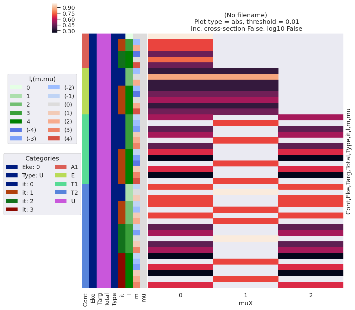
lmPlot

[9]:

# Print values (from matE data) with lmPlot
data.lmPlot(xDim = 'muX')

/home/femtolab/anaconda3/envs/epsdev-030821/lib/python3.7/site-packages/xarray/core/nputils.py:223: RuntimeWarning: All-NaN slice encountered
  result = getattr(npmodule, name)(values, axis=axis, **kwargs)

Plotting data (No filename), pType=a, thres=0.01, with Seaborn

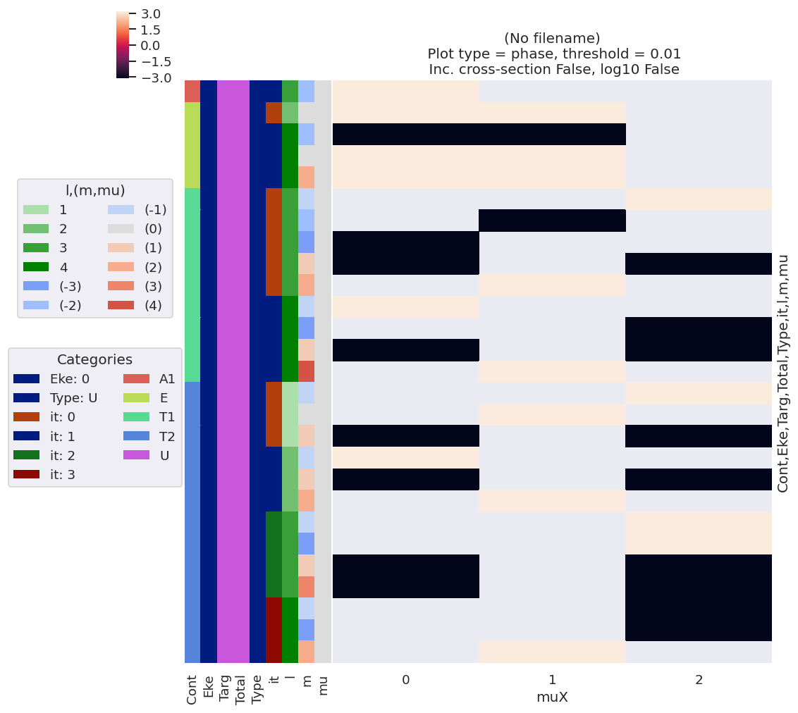
../_images/sym_pemtk_symHarm_epsproc-interface_demo_240322_18_2.png

[11]:

# Phase info
data.lmPlot(xDim = 'muX', pType='phase')

/home/femtolab/anaconda3/envs/epsdev-030821/lib/python3.7/site-packages/xarray/core/nputils.py:223: RuntimeWarning: All-NaN slice encountered
  result = getattr(npmodule, name)(values, axis=axis, **kwargs)

Plotting data (No filename), pType=phase, thres=0.01, with Seaborn

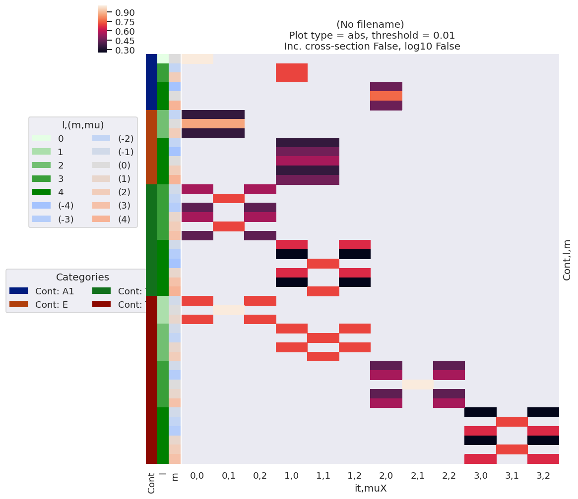
../_images/sym_pemtk_symHarm_epsproc-interface_demo_240322_19_2.png

[31]:

# Plot by label sets with a dim mapping & drop singleton dims with squeeze
data.lmPlot(xDim = {'X':['it','muX']}, squeeze = True, pType='a')

/home/femtolab/anaconda3/envs/epsdev-030821/lib/python3.7/site-packages/xarray/core/nputils.py:223: RuntimeWarning: All-NaN slice encountered
  result = getattr(npmodule, name)(values, axis=axis, **kwargs)

Plotting data (No filename), pType=a, thres=0.01, with Seaborn

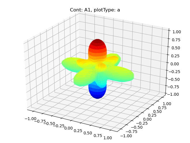
../_images/sym_pemtk_symHarm_epsproc-interface_demo_240322_20_2.png

padPlot

This has some basic functionality for polar plots.

[12]:

# Plot full harmonics expansions, plots by symmetry
# Note 'squeeze=True' to force drop of singleton dims may be required.
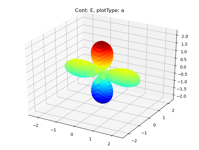
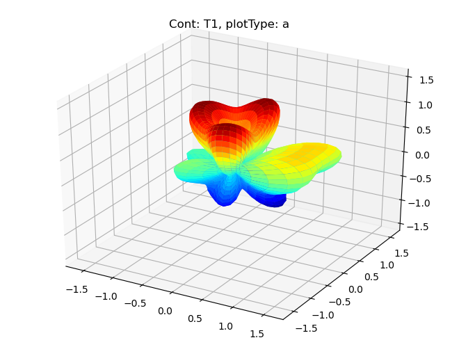
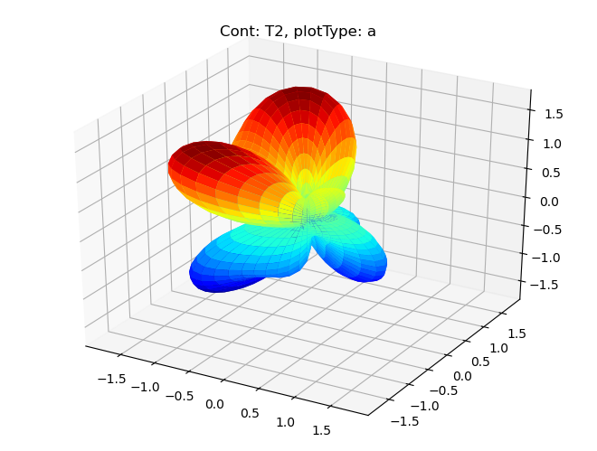
data.padPlot(dataType='BLM', facetDims = ['Cont'], squeeze = True)

Using default sph betas.
Summing over dims: {'it'}
Found additional dims {'muX'}, summing to reduce for plot. Pass selDims to avoid.
Sph plots: Cont: A1, plotType: a
Plotting with mpl
Sph plots: Cont: E, plotType: a
Plotting with mpl
Sph plots: Cont: T1, plotType: a
Plotting with mpl
Sph plots: Cont: T2, plotType: a
Plotting with mpl

../_images/sym_pemtk_symHarm_epsproc-interface_demo_240322_22_1.png

../_images/sym_pemtk_symHarm_epsproc-interface_demo_240322_22_2.png

../_images/sym_pemtk_symHarm_epsproc-interface_demo_240322_22_3.png

../_images/sym_pemtk_symHarm_epsproc-interface_demo_240322_22_4.png

[14]:

# Single symmetry by degenerate components
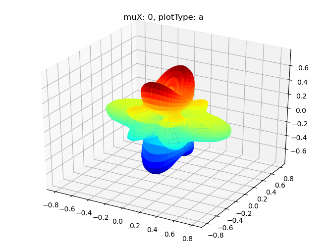
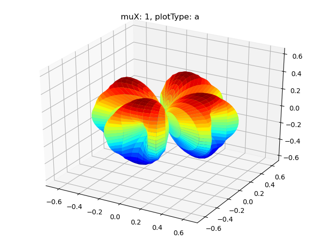
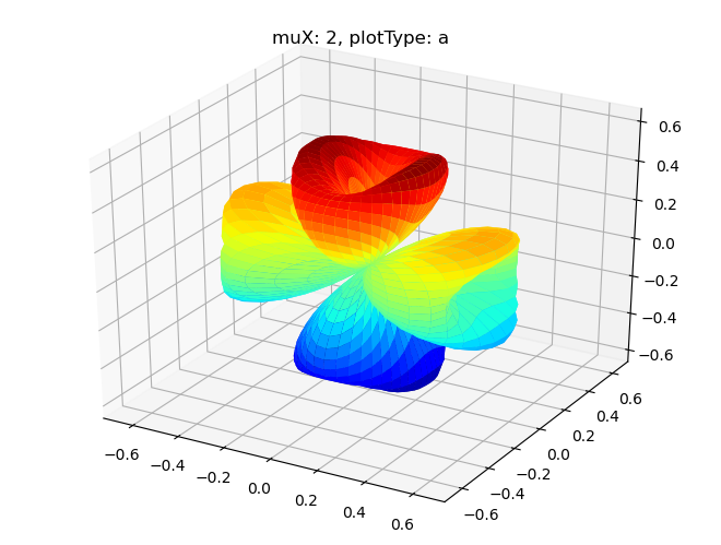
data.padPlot(dataType='BLM', selDims = {'Cont':'T1'}, facetDims = ['muX'], pType = 'a')

Using default sph betas.
Summing over dims: {'it'}
Found additional dims {'Eke', 'Euler'}, summing to reduce for plot. Pass selDims to avoid.
Sph plots: muX: 0, plotType: a
Plotting with mpl
Sph plots: muX: 1, plotType: a
Plotting with mpl
Sph plots: muX: 2, plotType: a
Plotting with mpl

../_images/sym_pemtk_symHarm_epsproc-interface_demo_240322_23_1.png

../_images/sym_pemtk_symHarm_epsproc-interface_demo_240322_23_2.png

../_images/sym_pemtk_symHarm_epsproc-interface_demo_240322_23_3.png

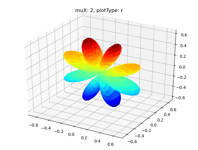
[15]:

# Single symmetry by degenerate components - real part
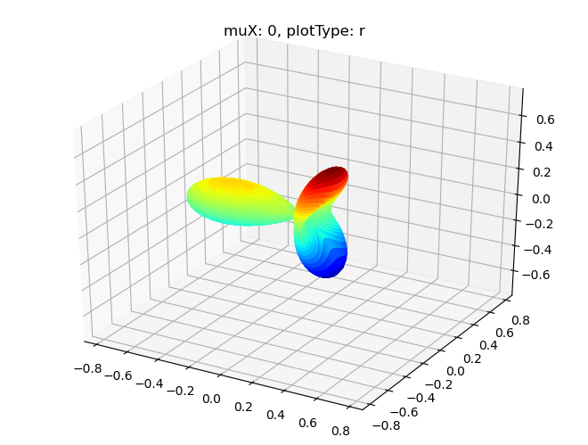
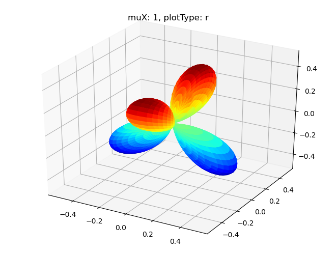
data.padPlot(dataType='BLM', selDims = {'Cont':'T1'}, facetDims = ['muX'], pType = 'r')

Using default sph betas.
Summing over dims: {'it'}
Found additional dims {'Eke', 'Euler'}, summing to reduce for plot. Pass selDims to avoid.
Sph plots: muX: 0, plotType: r
Plotting with mpl
Sph plots: muX: 1, plotType: r
Plotting with mpl
Sph plots: muX: 2, plotType: r
Plotting with mpl

../_images/sym_pemtk_symHarm_epsproc-interface_demo_240322_24_1.png

../_images/sym_pemtk_symHarm_epsproc-interface_demo_240322_24_2.png

../_images/sym_pemtk_symHarm_epsproc-interface_demo_240322_24_3.png

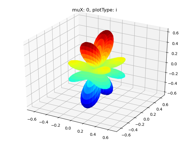
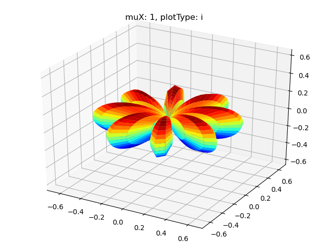
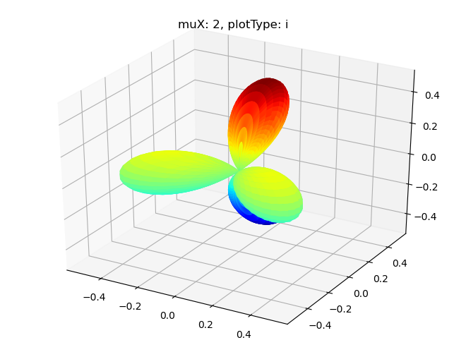
[16]:

# Single symmetry by degenerate components - imag part
data.padPlot(dataType='BLM', selDims = {'Cont':'T1'}, facetDims = ['muX'], pType = 'i')

Using default sph betas.
Summing over dims: {'it'}
Found additional dims {'Eke', 'Euler'}, summing to reduce for plot. Pass selDims to avoid.
Sph plots: muX: 0, plotType: i
Plotting with mpl
Sph plots: muX: 1, plotType: i
Plotting with mpl
Sph plots: muX: 2, plotType: i
Plotting with mpl

../_images/sym_pemtk_symHarm_epsproc-interface_demo_240322_25_1.png

../_images/sym_pemtk_symHarm_epsproc-interface_demo_240322_25_2.png

../_images/sym_pemtk_symHarm_epsproc-interface_demo_240322_25_3.png

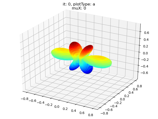
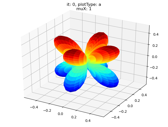
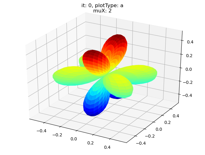
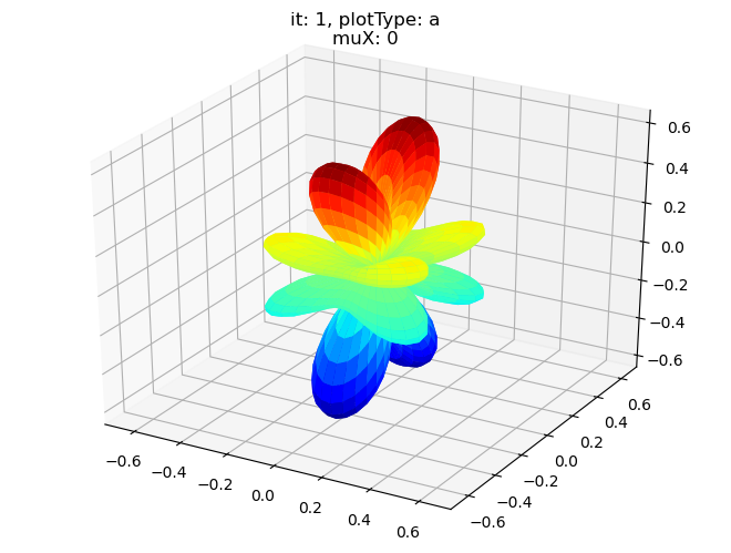
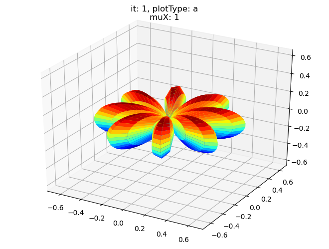
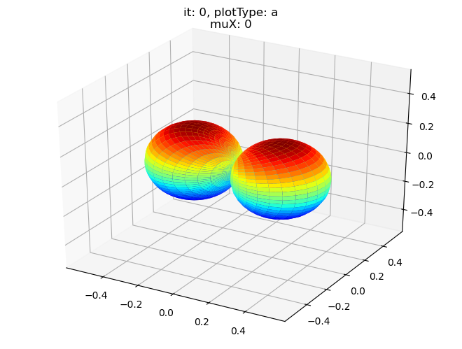
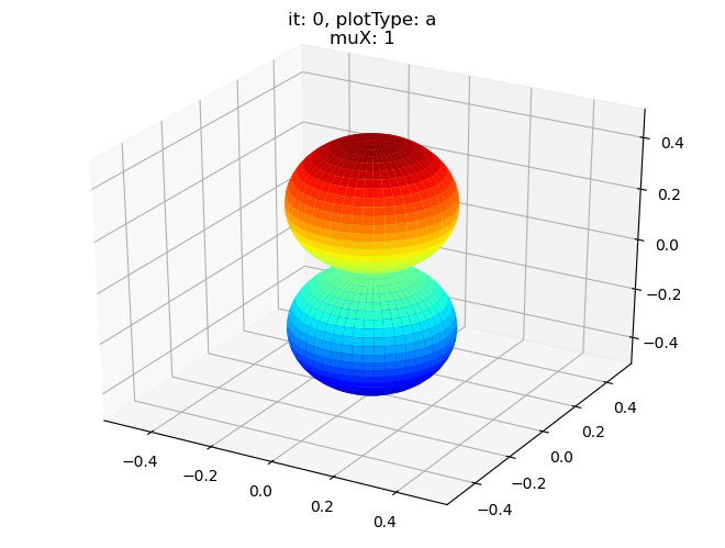
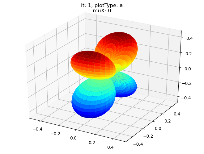
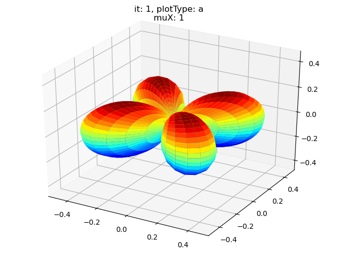
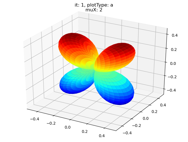
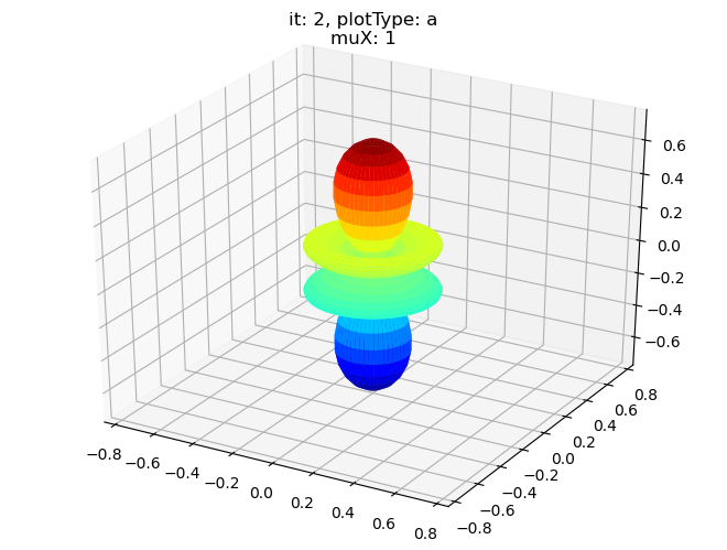
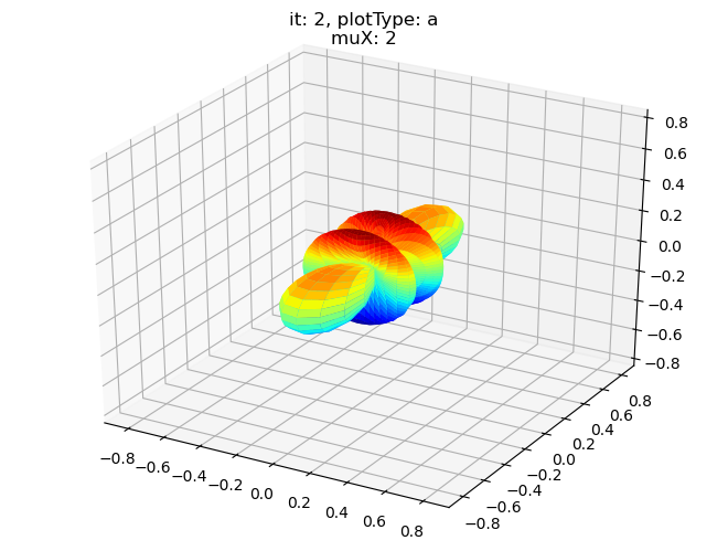
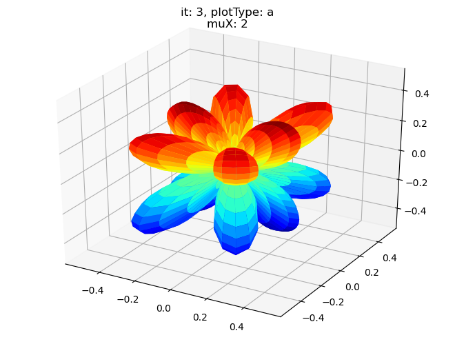
[18]:

# Single symmetry by degenerate components - real part, all components
# Note this currently requires sumDims = {}
# TODO: Also should be able to drop empty cases? Maybe set thres?
data.padPlot(dataType='BLM', selDims = {'Cont':'T1'}, sumDims = {}, facetDims = ['it','muX'], pType = 'a')

Using default sph betas.
Found additional dims {'Eke', 'Euler'}, summing to reduce for plot. Pass selDims to avoid.
Sph plots: it: 0, plotType: a
Plotting with mpl
Data dims: ('muX', 'Phi', 'Theta'), subplots on muX
Sph plots: it: 1, plotType: a
Plotting with mpl
Data dims: ('muX', 'Phi', 'Theta'), subplots on muX
Sph plots: it: 2, plotType: a
Plotting with mpl
Data dims: ('muX', 'Phi', 'Theta'), subplots on muX
Sph plots: it: 3, plotType: a
Plotting with mpl
Data dims: ('muX', 'Phi', 'Theta'), subplots on muX

../_images/sym_pemtk_symHarm_epsproc-interface_demo_240322_26_1.png

../_images/sym_pemtk_symHarm_epsproc-interface_demo_240322_26_2.png

../_images/sym_pemtk_symHarm_epsproc-interface_demo_240322_26_3.png

../_images/sym_pemtk_symHarm_epsproc-interface_demo_240322_26_4.png

../_images/sym_pemtk_symHarm_epsproc-interface_demo_240322_26_5.png

../_images/sym_pemtk_symHarm_epsproc-interface_demo_240322_26_6.png

../_images/sym_pemtk_symHarm_epsproc-interface_demo_240322_26_7.png

../_images/sym_pemtk_symHarm_epsproc-interface_demo_240322_26_8.png

../_images/sym_pemtk_symHarm_epsproc-interface_demo_240322_26_9.png

../_images/sym_pemtk_symHarm_epsproc-interface_demo_240322_26_10.png

../_images/sym_pemtk_symHarm_epsproc-interface_demo_240322_26_11.png

../_images/sym_pemtk_symHarm_epsproc-interface_demo_240322_26_12.png

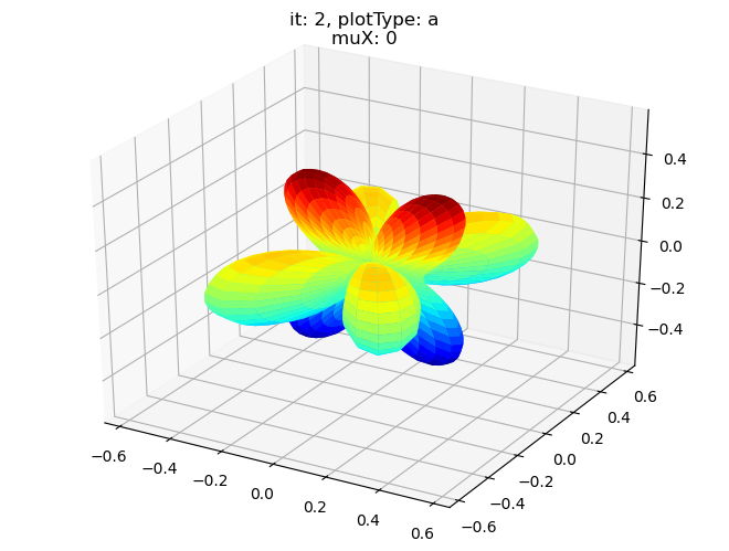
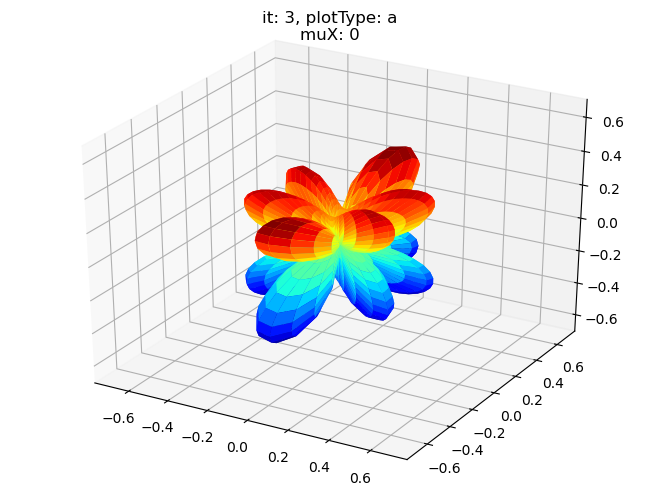
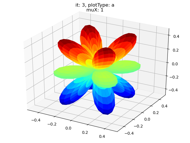
[19]:

data.padPlot(dataType='BLM', selDims = {'Cont':'T2'}, sumDims = {}, facetDims = ['it','muX'], pType = 'a')

Using default sph betas.
Found additional dims {'Eke', 'Euler'}, summing to reduce for plot. Pass selDims to avoid.
Sph plots: it: 0, plotType: a
Plotting with mpl
Data dims: ('muX', 'Phi', 'Theta'), subplots on muX
Sph plots: it: 1, plotType: a
Plotting with mpl
Data dims: ('muX', 'Phi', 'Theta'), subplots on muX
Sph plots: it: 2, plotType: a
Plotting with mpl
Data dims: ('muX', 'Phi', 'Theta'), subplots on muX
Sph plots: it: 3, plotType: a
Plotting with mpl
Data dims: ('muX', 'Phi', 'Theta'), subplots on muX

../_images/sym_pemtk_symHarm_epsproc-interface_demo_240322_27_1.png

../_images/sym_pemtk_symHarm_epsproc-interface_demo_240322_27_2.png

../_images/sym_pemtk_symHarm_epsproc-interface_demo_240322_27_3.png

../_images/sym_pemtk_symHarm_epsproc-interface_demo_240322_27_4.png

../_images/sym_pemtk_symHarm_epsproc-interface_demo_240322_27_5.png

../_images/sym_pemtk_symHarm_epsproc-interface_demo_240322_27_6.png

../_images/sym_pemtk_symHarm_epsproc-interface_demo_240322_27_7.png

../_images/sym_pemtk_symHarm_epsproc-interface_demo_240322_27_8.png

../_images/sym_pemtk_symHarm_epsproc-interface_demo_240322_27_9.png

../_images/sym_pemtk_symHarm_epsproc-interface_demo_240322_27_10.png

../_images/sym_pemtk_symHarm_epsproc-interface_demo_240322_27_11.png

../_images/sym_pemtk_symHarm_epsproc-interface_demo_240322_27_12.png

ePSproc density matrix functionality

Functions following https://epsproc.readthedocs.io/en/dev/methods/density_mat_notes_demo_300821.html

Still in development.

[21]:

# Import routines
from epsproc.calc import density

[22]:

# Set data from master class (routines not yet wrapped)
k = 'symHarm'  # N2 orb5 (SG) dataset
matE = data.data[k]['matE']
# selDims = {'Type':'L'}
selDims = {}
thres = 1e-2

[25]:

# Compose density matrix

# Set dimensions/state vector/representation
# These must be in original data, but will be restacked as necessary to define the effective basis space.
denDims = ['LM', 'muX', 'it']

# Calculate
daOut, *_ = density.densityCalc(matE, denDims = denDims, selDims = selDims, thres = thres)  # OK

[45]:

# Plot full matrix
# This is interactive (with Holoviews), with the widgets allowing selection of other (stacked) dimensions.
# Plot types [real, imag, abs] are also set.
# Note this may take a while for data with a large number of dimensions.

# density.matPlot(daOut)
# density.matPlot(daOut.sel({'Cont':'A1'}).squeeze())  # Specific symmetry

# NOTE - not currently working on bemo in epsdev-030821 env, looks like HV version rendering issue?

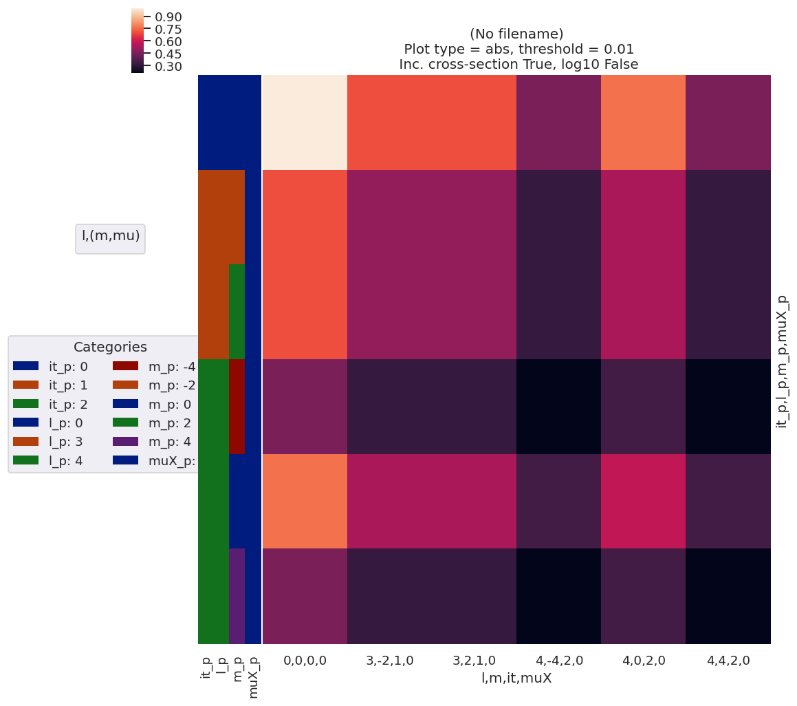
[41]:

# Use lmPlot to show the full dimensionality
# Note for mixed stacked + unstacked denDims, may need to specify manually (unstacked dims only)
ep.lmPlot(daOut.sel({'Cont':'A1'}).squeeze(), xDim={'den':['l','m','it','muX']});   #{'den':denDims});

/home/femtolab/anaconda3/envs/epsdev-030821/lib/python3.7/site-packages/xarray/core/nputils.py:223: RuntimeWarning: All-NaN slice encountered
  result = getattr(npmodule, name)(values, axis=axis, **kwargs)

Plotting data (No filename), pType=a, thres=0.01, with Seaborn

No handles with labels found to put in legend.

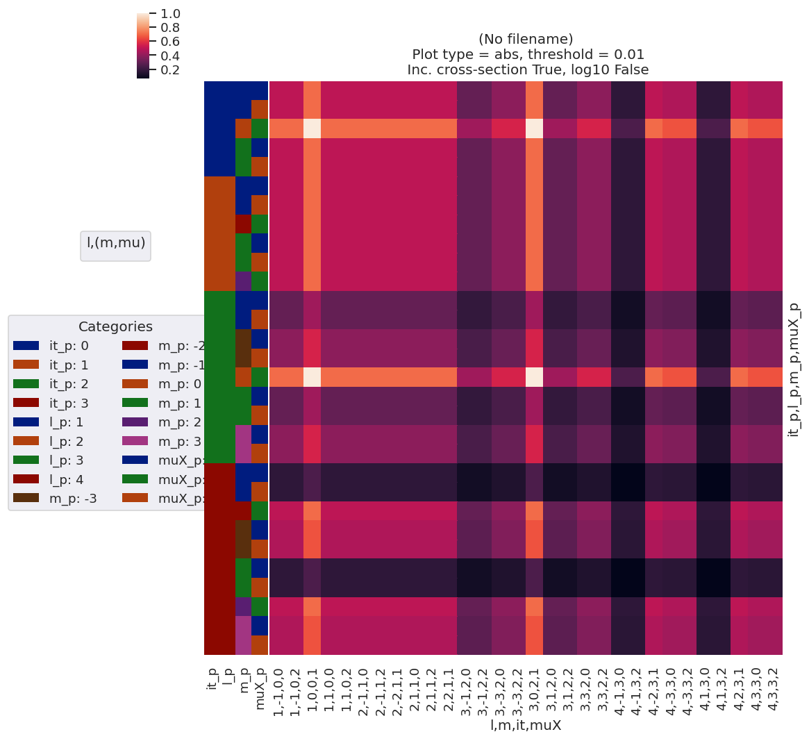
../_images/sym_pemtk_symHarm_epsproc-interface_demo_240322_33_3.png

[42]:

ep.lmPlot(daOut.sel({'Cont':'T2'}).squeeze(), xDim={'den':['l','m','it','muX']});   #{'den':denDims});

/home/femtolab/anaconda3/envs/epsdev-030821/lib/python3.7/site-packages/xarray/core/nputils.py:223: RuntimeWarning: All-NaN slice encountered
  result = getattr(npmodule, name)(values, axis=axis, **kwargs)

Plotting data (No filename), pType=a, thres=0.01, with Seaborn

No handles with labels found to put in legend.

../_images/sym_pemtk_symHarm_epsproc-interface_demo_240322_34_3.png

Versions

[19]:

import scooby
scooby.Report(additional=['epsproc', 'pemtk', 'holoviews', 'hvplot', 'xarray', 'matplotlib', 'bokeh', 'pyshtools'])

[19]:

Thu Mar 24 12:20:09 2022 EDT
OS	Linux	CPU(s)	4	Machine	x86_64
Architecture	64bit	RAM	7.7 GB	Environment	Jupyter
Python 3.7.6 (default, Jan 8 2020, 19:59:22) [GCC 7.3.0]
epsproc	1.3.1-dev	pemtk	0.0.1	holoviews	1.12.6
hvplot	0.6.0	xarray	0.13.0	matplotlib	3.2.0
bokeh	1.4.0	pyshtools	4.5	numpy	1.18.1
scipy	1.3.1	IPython	7.13.0	scooby	0.5.5
Intel(R) Math Kernel Library Version 2019.0.4 Product Build 20190411 for Intel(R) 64 architecture applications

[20]:

# Check current Git commit for local ePSproc version
import pemtk
from pathlib import Path
!git -C {Path(pemtk.__file__).parent} branch
!git -C {Path(pemtk.__file__).parent} log --format="%H" -n 1

* master
6c603e299dcfeb05ea730f415a35a604c964d193

[21]:

# Check current remote commits
!git ls-remote --heads https://github.com/phockett/pemtk

6c603e299dcfeb05ea730f415a35a604c964d193        refs/heads/master

[20]:

# Check current Git commit for local ePSproc version
import epsproc
from pathlib import Path
!git -C {Path(epsproc.__file__).parent} branch
!git -C {Path(epsproc.__file__).parent} log --format="%H" -n 1

* master
6c603e299dcfeb05ea730f415a35a604c964d193

[21]:

# Check current remote commits
!git ls-remote --heads https://github.com/phockett/epsproc

6c603e299dcfeb05ea730f415a35a604c964d193        refs/heads/master