06/12/21 - TO FIX: push/debug ePSproc updates, currently throwing loading errors on Jake
Analysis routines
06/12/21 v2 with updated param analysis and tabulation routines.
14/11/21 v1 (still in development)
In this notebook some of the packaged analysis routines are demonstrated. For an earlier exploration of the basic/underlying analysis routines, see the previous fit fidelity & analysis notebook.
Setup
Load fit & analysis class and import data (currently a bit messy).
[1]:
# Import & set paths
import pemtk
from pemtk.fit.fitClass import pemtkFit
from pathlib import Path
# Path for demo script
demoPath = Path(pemtk.__file__).parent.parent/Path('demos','fitting')
# Some additional default plot settings
# TODO: this is already run at class init, but out of notebook scope? Should fix.
from epsproc.plot import hvPlotters
hvPlotters.setPlotters()
*** ePSproc installation not found, setting for local copy.


C:\Users\femtolab\.conda\envs\ePSdev\lib\importlib\_bootstrap.py:219: RuntimeWarning: numpy.ufunc size changed, may indicate binary incompatibility. Expected 192 from C header, got 216 from PyObject
return f(*args, **kwds)
C:\Users\femtolab\.conda\envs\ePSdev\lib\site-packages\xyzpy\plot\xyz_cmaps.py:6: MatplotlibDeprecationWarning:
The revcmap function was deprecated in Matplotlib 3.2 and will be removed two minor releases later. Use Colormap.reversed() instead.
return LinearSegmentedColormap(name, cm.revcmap(cmap._segmentdata))
[2]:
# Here we'll just load some test data
# TODO: wrap this to class!
# Load sample dataset
# Full path to the file may be required here, in repo/demos/fitting
import pickle
from pathlib import Path
# dataPath = Path(pemtk.__path__[0]).parent/Path('demos','fitting') # Test data in repo
dataPath = demoPath
# Basic test data - simulated results with no noise, 100 fits
# dataFile = 'dataDump_100fitTests_10t_randPhase_130621.pickle'
# Noisey test data - simulated results with noise, 1000 fits
dataFile = 'dataDump_1000fitTests_multiFit_noise_051021.pickle'
# Set for empty class, or with full demo setup (includes ref. parameter set)
demo = False
if demo:
# Version with full demo setup
%run {demoPath/"setup_fit_demo.py"}
else:
data = pemtkFit() # Data loads OK for blank class, but may be missing some necessary vars.
data.verbose['sub'] = 1
with open( dataPath/dataFile, 'rb') as handle:
data.data = pickle.load(handle)
data.fitInd = list(data.data.keys())[-1] # Set final key from data - probably not a robust method however!
# This is currently used for indexing
Data overview
For more on the data structures used here, see the setup & batch runs notebook.
[3]:
# Check number of datasets loaded
data.fitInd
[3]:
999
[4]:
# Run basic stats
# TODO: add more outputs here & tidy up output formatting.
data.analyseFits()
Pandas reference table not set, missing self.params data.
Setting wide-form data self.[fits][dfWide] from self.[fits][dfLong] (as pivot table).
*** Warning: found MultiIndex for DataFrame data.index - checkDims doesn't yet support Pandas MultiIndex.
*** Warning: found MultiIndex for DataFrame data.index - checkDims doesn't yet support Pandas MultiIndex.
Index(es) = ['Fit', 'Type'], cols = value
{ 'Fits': 999,
'Minima': {'chisqr': 0.04215746268613921, 'redchi': 0.00022911664503336526},
'Success': 991}
[5]:
# Basic histogram of fit sets
# Note this defaults to Holoviews/Bokeh for plotting, which produces an interactive plot.
# Set backend = 'mpl' if Holoviews is not available.
data.fitHist()
The overview histogram is fairly coarse, since it shows all results. It is clear, however, that there are many results at the low end of the range (by default this plots reduced \(\chi^2\) values). This can be explored in further detail via the interactive plot (if using Holoviews), or via further plotting with specified thresholds or ranges (see below).
Dataset notes:
For “perfect” data (
dataDump_1000fitTests_multiFit_130921.pickle) can get a large spread here, with best results at \(10^{-11}\).For noisey data (
dataDump_1000fitTests_multiFit_noise_011021.pickle) have a smaller spread, best results low \(10^{-4}\).
[6]:
# With threshold set & fine binning.
# See fitHist() docs for more options.
data.fitHist(thres = 2.4e-4, bins = 100)
# data.fitHist(bins=20, binRange = [2.3e-4, 2.4e-4]) # Example with a range set
Mask selected 561 results (from 999).
Data exploration
The general aim in this procedure is to ascertain whether there was a good spread of parameters explored, and a single (or few sets) of best-fit results. There are a few procedures and helper methods for this…
View results
Single results sets can be viewed in the main data structure, indexed by #.
[7]:
# Check keys
fitNumber = 2
data.data[fitNumber].keys()
[7]:
dict_keys(['AFBLM', 'residual', 'results'])
Here results is an lmFit object, which includes final fit results and information, and AFBLM contains the model output. (TODO: helper functions for this.)
An example is shown below. Of particular note here is which parameters have vary=True - these are included in the fitting - and if there is a column expression, which indicates any parameters defined to have specific relationships (see the basic demo notebook for more). Any correlations found during fitting are also shown, which can also indicate
parameters which are related (even if this is not predefined or known a priori).
For the current dataset (‘dataDump_1000fitTests_multiFit_noise_051021.pickle’), note that p_PU_SG_PU_1_n1_1_1 has vary=False, hence the results are already defined as relative phases (and, in this example, the fixed value is kept at the original model value).
[8]:
# Show some results
data.data[fitNumber]['results']
[8]:
Fit Statistics
| fitting method | leastsq | |
| # function evals | 2812 | |
| # data points | 195 | |
| # variables | 11 | |
| chi-square | 0.04215747 | |
| reduced chi-square | 2.2912e-04 | |
| Akaike info crit. | -1623.67186 | |
| Bayesian info crit. | -1587.66886 |
Variables
| name | value | standard error | relative error | initial value | min | max | vary |
|---|---|---|---|---|---|---|---|
| m_PU_SG_PU_1_n1_1_1 | 1.61758339 | 227151.843 | (14042666.65%) | 0.4963375310160162 | 1.0000e-04 | 5.00000000 | True |
| m_PU_SG_PU_1_1_n1_1 | 1.60986876 | 227266.217 | (14117064.81%) | 0.349972501184159 | 1.0000e-04 | 5.00000000 | True |
| m_PU_SG_PU_3_n1_1_1 | 1.14366717 | 214620.511 | (18765993.77%) | 0.43544003283291643 | 1.0000e-04 | 5.00000000 | True |
| m_PU_SG_PU_3_1_n1_1 | 1.14104307 | 213989.161 | (18753819.79%) | 0.16101762796183416 | 1.0000e-04 | 5.00000000 | True |
| m_SU_SG_SU_1_0_0_1 | 2.65253557 | 0.06899386 | (2.60%) | 0.8234700291388766 | 1.0000e-04 | 5.00000000 | True |
| m_SU_SG_SU_3_0_0_1 | 1.14378960 | 0.14902324 | (13.03%) | 0.5411867072477154 | 1.0000e-04 | 5.00000000 | True |
| p_PU_SG_PU_1_n1_1_1 | -0.86104140 | 0.00000000 | (0.00%) | -0.8610414024232179 | -3.14159265 | 3.14159265 | False |
| p_PU_SG_PU_1_1_n1_1 | -0.85729904 | 167895.839 | (19584279.35%) | 0.021992539259326538 | -3.14159265 | 3.14159265 | True |
| p_PU_SG_PU_3_n1_1_1 | 1.20005808 | 224407.741 | (18699740.07%) | 0.023782497271738423 | -3.14159265 | 3.14159265 | True |
| p_PU_SG_PU_3_1_n1_1 | 1.19902071 | 296532.682 | (24731239.48%) | 0.5554954153030479 | -3.14159265 | 3.14159265 | True |
| p_SU_SG_SU_1_0_0_1 | 2.43703747 | 83742.0262 | (3436222.35%) | 0.5266569153447359 | -3.14159265 | 3.14159265 | True |
| p_SU_SG_SU_3_0_0_1 | -0.70401900 | 83725.8242 | (11892551.81%) | 0.004178913362662073 | -3.14159265 | 3.14159265 | True |
Correlations (unreported correlations are < 0.100)
| m_PU_SG_PU_1_n1_1_1 | m_PU_SG_PU_1_1_n1_1 | -1.0000 |
| m_PU_SG_PU_3_n1_1_1 | m_PU_SG_PU_3_1_n1_1 | -1.0000 |
| p_SU_SG_SU_1_0_0_1 | p_SU_SG_SU_3_0_0_1 | 1.0000 |
| p_PU_SG_PU_1_1_n1_1 | p_SU_SG_SU_1_0_0_1 | 0.9999 |
| p_PU_SG_PU_1_1_n1_1 | p_SU_SG_SU_3_0_0_1 | 0.9999 |
| m_PU_SG_PU_3_n1_1_1 | p_PU_SG_PU_3_n1_1_1 | 0.9923 |
| m_PU_SG_PU_3_1_n1_1 | p_PU_SG_PU_3_n1_1_1 | -0.9921 |
| m_PU_SG_PU_1_n1_1_1 | m_PU_SG_PU_3_1_n1_1 | 0.9852 |
| m_PU_SG_PU_1_n1_1_1 | m_PU_SG_PU_3_n1_1_1 | -0.9849 |
| m_PU_SG_PU_1_1_n1_1 | m_PU_SG_PU_3_1_n1_1 | -0.9848 |
| m_PU_SG_PU_1_1_n1_1 | m_PU_SG_PU_3_n1_1_1 | 0.9845 |
| m_PU_SG_PU_1_n1_1_1 | p_PU_SG_PU_3_n1_1_1 | -0.9585 |
| m_PU_SG_PU_1_1_n1_1 | p_PU_SG_PU_3_n1_1_1 | 0.9579 |
| m_SU_SG_SU_1_0_0_1 | m_SU_SG_SU_3_0_0_1 | -0.9312 |
| p_PU_SG_PU_3_n1_1_1 | p_PU_SG_PU_3_1_n1_1 | -0.8223 |
| m_PU_SG_PU_3_n1_1_1 | p_PU_SG_PU_3_1_n1_1 | -0.7514 |
| m_PU_SG_PU_3_1_n1_1 | p_PU_SG_PU_3_1_n1_1 | 0.7503 |
| p_PU_SG_PU_1_1_n1_1 | p_PU_SG_PU_3_1_n1_1 | 0.6663 |
| p_PU_SG_PU_3_1_n1_1 | p_SU_SG_SU_1_0_0_1 | 0.6480 |
| p_PU_SG_PU_3_1_n1_1 | p_SU_SG_SU_3_0_0_1 | 0.6476 |
| m_PU_SG_PU_1_n1_1_1 | p_PU_SG_PU_3_1_n1_1 | 0.6332 |
| m_PU_SG_PU_1_1_n1_1 | p_PU_SG_PU_3_1_n1_1 | -0.6316 |
| m_PU_SG_PU_3_n1_1_1 | m_SU_SG_SU_1_0_0_1 | -0.5284 |
| m_PU_SG_PU_3_1_n1_1 | m_SU_SG_SU_1_0_0_1 | 0.5284 |
| m_SU_SG_SU_1_0_0_1 | p_PU_SG_PU_3_n1_1_1 | -0.5263 |
| m_PU_SG_PU_1_n1_1_1 | m_SU_SG_SU_1_0_0_1 | 0.5166 |
| m_PU_SG_PU_1_1_n1_1 | m_SU_SG_SU_1_0_0_1 | -0.5164 |
| m_PU_SG_PU_3_n1_1_1 | m_SU_SG_SU_3_0_0_1 | 0.4968 |
| m_PU_SG_PU_3_1_n1_1 | m_SU_SG_SU_3_0_0_1 | -0.4967 |
| m_SU_SG_SU_3_0_0_1 | p_PU_SG_PU_3_n1_1_1 | 0.4949 |
| m_PU_SG_PU_1_n1_1_1 | m_SU_SG_SU_3_0_0_1 | -0.4853 |
| m_PU_SG_PU_1_1_n1_1 | m_SU_SG_SU_3_0_0_1 | 0.4851 |
| m_SU_SG_SU_1_0_0_1 | p_PU_SG_PU_3_1_n1_1 | 0.4101 |
| m_SU_SG_SU_3_0_0_1 | p_PU_SG_PU_3_1_n1_1 | -0.3865 |
| m_PU_SG_PU_1_1_n1_1 | p_SU_SG_SU_3_0_0_1 | 0.1724 |
| m_PU_SG_PU_1_1_n1_1 | p_SU_SG_SU_1_0_0_1 | 0.1719 |
| m_PU_SG_PU_1_n1_1_1 | p_SU_SG_SU_3_0_0_1 | -0.1702 |
| m_PU_SG_PU_1_n1_1_1 | p_SU_SG_SU_1_0_0_1 | -0.1697 |
| m_PU_SG_PU_1_1_n1_1 | p_PU_SG_PU_1_1_n1_1 | 0.1670 |
| m_PU_SG_PU_1_n1_1_1 | p_PU_SG_PU_1_1_n1_1 | -0.1648 |
| p_PU_SG_PU_1_1_n1_1 | p_PU_SG_PU_3_n1_1_1 | -0.1330 |
| p_PU_SG_PU_3_n1_1_1 | p_SU_SG_SU_1_0_0_1 | -0.1088 |
| p_PU_SG_PU_3_n1_1_1 | p_SU_SG_SU_3_0_0_1 | -0.1083 |
Classify fits
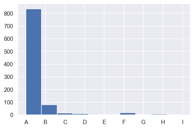
To review and classify the “sets” of fit results which are apparent here, use the classifyFits() method. This will rebin/categorise the data and label each bin alphabetically.
[9]:
# The default case simply rebins all data into 10 categories.
data.classifyFits()
| success | chisqr | redchi | Min | Max | ||||||||||
|---|---|---|---|---|---|---|---|---|---|---|---|---|---|---|
| count | unique | top | freq | count | unique | top | freq | count | unique | top | freq | |||
| redchiGroup | ||||||||||||||
| A | 835 | 2 | True | 833 | 835.0 | 835.0 | 0.044630 | 1.0 | 835.0 | 835.0 | 0.000229 | 1.0 | 0.000218 | 0.000321 |
| B | 80 | 2 | True | 79 | 80.0 | 80.0 | 0.069253 | 1.0 | 80.0 | 80.0 | 0.000377 | 1.0 | 0.000321 | 0.000424 |
| C | 14 | 2 | True | 13 | 14.0 | 14.0 | 0.088500 | 1.0 | 14.0 | 14.0 | 0.000440 | 1.0 | 0.000424 | 0.000527 |
| D | 11 | 1 | True | 11 | 11.0 | 11.0 | 0.103048 | 1.0 | 11.0 | 11.0 | 0.000605 | 1.0 | 0.000527 | 0.000630 |
| E | 6 | 1 | True | 6 | 6.0 | 6.0 | 0.132356 | 1.0 | 6.0 | 6.0 | 0.000719 | 1.0 | 0.000630 | 0.000733 |
| F | 18 | 1 | True | 18 | 18.0 | 18.0 | 0.140435 | 1.0 | 18.0 | 18.0 | 0.000775 | 1.0 | 0.000733 | 0.000836 |
| G | 4 | 1 | True | 4 | 4.0 | 4.0 | 0.154999 | 1.0 | 4.0 | 4.0 | 0.000842 | 1.0 | 0.000836 | 0.000939 |
| H | 7 | 1 | True | 7 | 7.0 | 7.0 | 0.173290 | 1.0 | 7.0 | 7.0 | 0.000942 | 1.0 | 0.000939 | 0.001042 |
| I | 2 | 1 | True | 2 | 2.0 | 2.0 | 0.193286 | 1.0 | 2.0 | 2.0 | 0.001053 | 1.0 | 0.001042 | 0.001146 |
Setting wide-form data self.[fits][dfWide] from self.[fits][dfLong] (as pivot table).
*** Warning: found MultiIndex for DataFrame data.index - checkDims doesn't yet support Pandas MultiIndex.
*** Warning: found MultiIndex for DataFrame data.index - checkDims doesn't yet support Pandas MultiIndex.
Index(es) = ['Fit', 'Type', 'redchiGroup'], cols = value
Set redchiGroup for data frame dfLong.
Set redchiGroup for data frame AFpdLong.
Couldn't set redchiGroup for data frame mask. Error <class 'KeyError'>: ('dType',).
[10]:
# Again, more control can be obtained by specifiying the desired binning.
data.classifyFits(bins = [2.26e-4, 2.4e-4,20])
| success | chisqr | redchi | Min | Max | ||||||||||
|---|---|---|---|---|---|---|---|---|---|---|---|---|---|---|
| count | unique | top | freq | count | unique | top | freq | count | unique | top | freq | |||
| redchiGroup | ||||||||||||||
| A | 0 | 0 | NaN | NaN | 0 | 0 | NaN | NaN | 0 | 0 | NaN | NaN | 0.000226 | 0.000227 |
| B | 0 | 0 | NaN | NaN | 0 | 0 | NaN | NaN | 0 | 0 | NaN | NaN | 0.000227 | 0.000227 |
| C | 0 | 0 | NaN | NaN | 0 | 0 | NaN | NaN | 0 | 0 | NaN | NaN | 0.000227 | 0.000228 |
| D | 0 | 0 | NaN | NaN | 0 | 0 | NaN | NaN | 0 | 0 | NaN | NaN | 0.000228 | 0.000229 |
| E | 349 | 1 | True | 349 | 349 | 349 | 0.0421575 | 1 | 349 | 349 | 0.000229117 | 1 | 0.000229 | 0.000230 |
| F | 0 | 0 | NaN | NaN | 0 | 0 | NaN | NaN | 0 | 0 | NaN | NaN | 0.000230 | 0.000230 |
| G | 27 | 1 | True | 27 | 27 | 27 | 0.0425252 | 1 | 27 | 27 | 0.000231115 | 1 | 0.000230 | 0.000231 |
| H | 43 | 1 | True | 43 | 43 | 43 | 0.0426516 | 1 | 43 | 43 | 0.000231163 | 1 | 0.000231 | 0.000232 |
| I | 24 | 1 | True | 24 | 24 | 24 | 0.0426877 | 1 | 24 | 24 | 0.000231998 | 1 | 0.000232 | 0.000233 |
| J | 0 | 0 | NaN | NaN | 0 | 0 | NaN | NaN | 0 | 0 | NaN | NaN | 0.000233 | 0.000233 |
| K | 11 | 1 | True | 11 | 11 | 11 | 0.0430736 | 1 | 11 | 11 | 0.000234096 | 1 | 0.000233 | 0.000234 |
| L | 27 | 1 | True | 27 | 27 | 27 | 0.0432038 | 1 | 27 | 27 | 0.000234803 | 1 | 0.000234 | 0.000235 |
| M | 3 | 2 | True | 2 | 3 | 3 | 0.0433464 | 1 | 3 | 3 | 0.000235579 | 1 | 0.000235 | 0.000236 |
| N | 54 | 1 | True | 54 | 54 | 54 | 0.0433468 | 1 | 54 | 54 | 0.000235581 | 1 | 0.000236 | 0.000236 |
| O | 5 | 1 | True | 5 | 5 | 5 | 0.0435333 | 1 | 5 | 5 | 0.00023659 | 1 | 0.000236 | 0.000237 |
| P | 0 | 0 | NaN | NaN | 0 | 0 | NaN | NaN | 0 | 0 | NaN | NaN | 0.000237 | 0.000238 |
| Q | 15 | 2 | True | 14 | 15 | 15 | 0.0438441 | 1 | 15 | 15 | 0.000237988 | 1 | 0.000238 | 0.000239 |
| R | 3 | 1 | True | 3 | 3 | 3 | 0.0439158 | 1 | 3 | 3 | 0.000238673 | 1 | 0.000239 | 0.000239 |
| S | 0 | 0 | NaN | NaN | 0 | 0 | NaN | NaN | 0 | 0 | NaN | NaN | 0.000239 | 0.000240 |
Setting wide-form data self.[fits][dfWide] from self.[fits][dfLong] (as pivot table).
*** Warning: found MultiIndex for DataFrame data.index - checkDims doesn't yet support Pandas MultiIndex.
*** Warning: found MultiIndex for DataFrame data.index - checkDims doesn't yet support Pandas MultiIndex.
Index(es) = ['Fit', 'Type', 'redchiGroup'], cols = value
Set redchiGroup for data frame dfLong.
Set redchiGroup for data frame AFpdLong.
Couldn't set redchiGroup for data frame mask. Error <class 'KeyError'>: ('dType',).
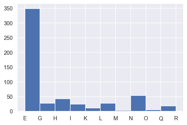
In this case, there are 349 fit results within the lowest (occupied) category (set E), which we can take to be the best fits possible in this case.
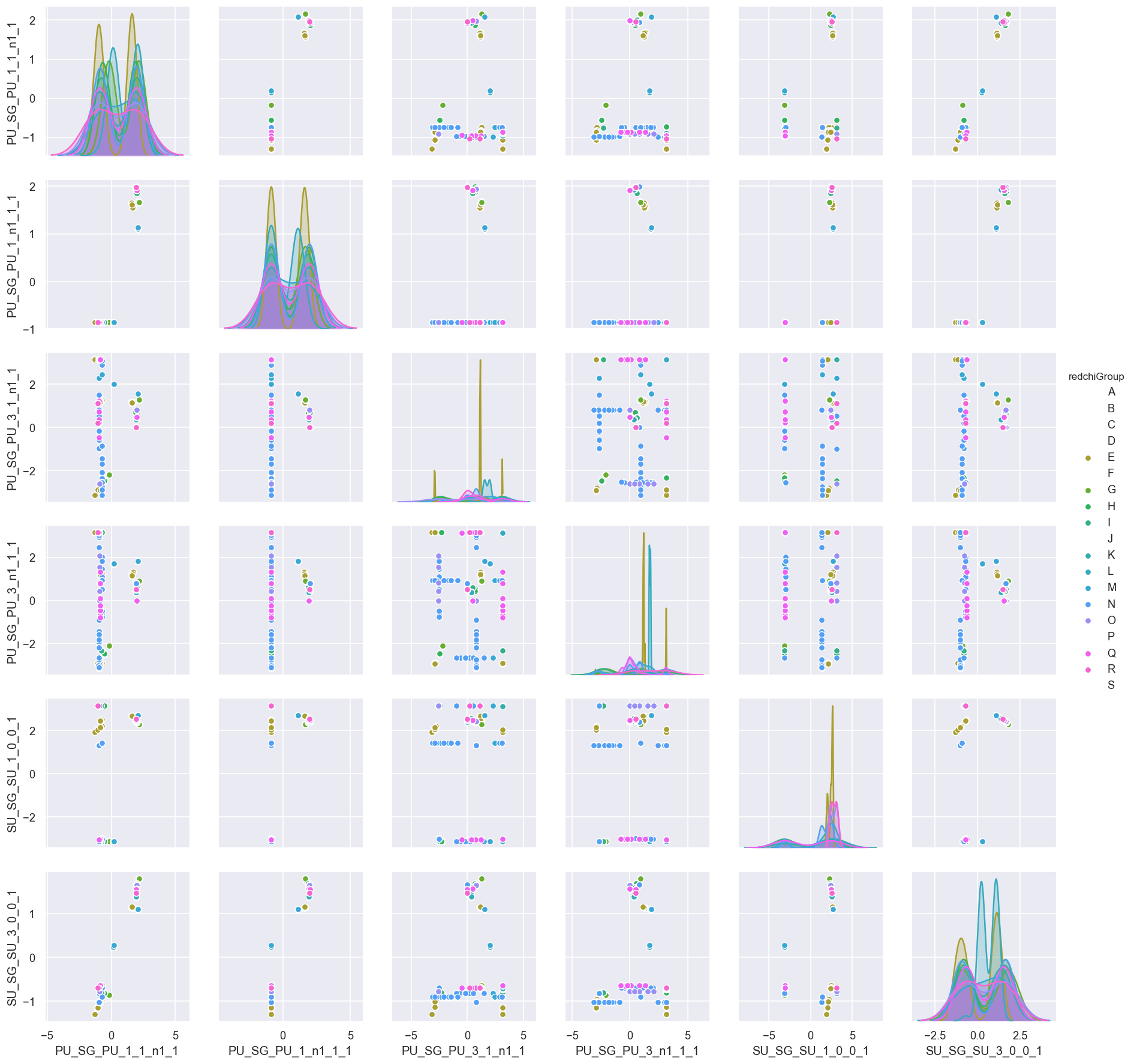
To visualise the associated parameter sets, we can use the corrPlot() and paramPlot() methods. These default to the currently set classified data (this is found in the wide-form data output by classifyFits(), which defaults to self.[fits][dfWide]), with colour-coding by group.
corrPlot()uses Seaborn’s pairplot routine to generate a full pair-wise correlation plot.paramPlot()uses Seaborn’s catplot routine to generate scatter plots for a specified data type.
corrPlot()
corrPlot() uses Seaborn’s pairplot routine to generate a full pair-wise correlation plot.
TODO: add HV gridmatrix + linked brushing: http://holoviews.org/user_guide/Linked_Brushing.html
[11]:
# Default plot will give output by grouping
data.corrPlot()
Mask not set for dataType = None.
*** Warning: found MultiIndex for DataFrame data.index - checkDims doesn't yet support Pandas MultiIndex.
<seaborn.axisgrid.PairGrid at 0x20519f5e048>
[12]:
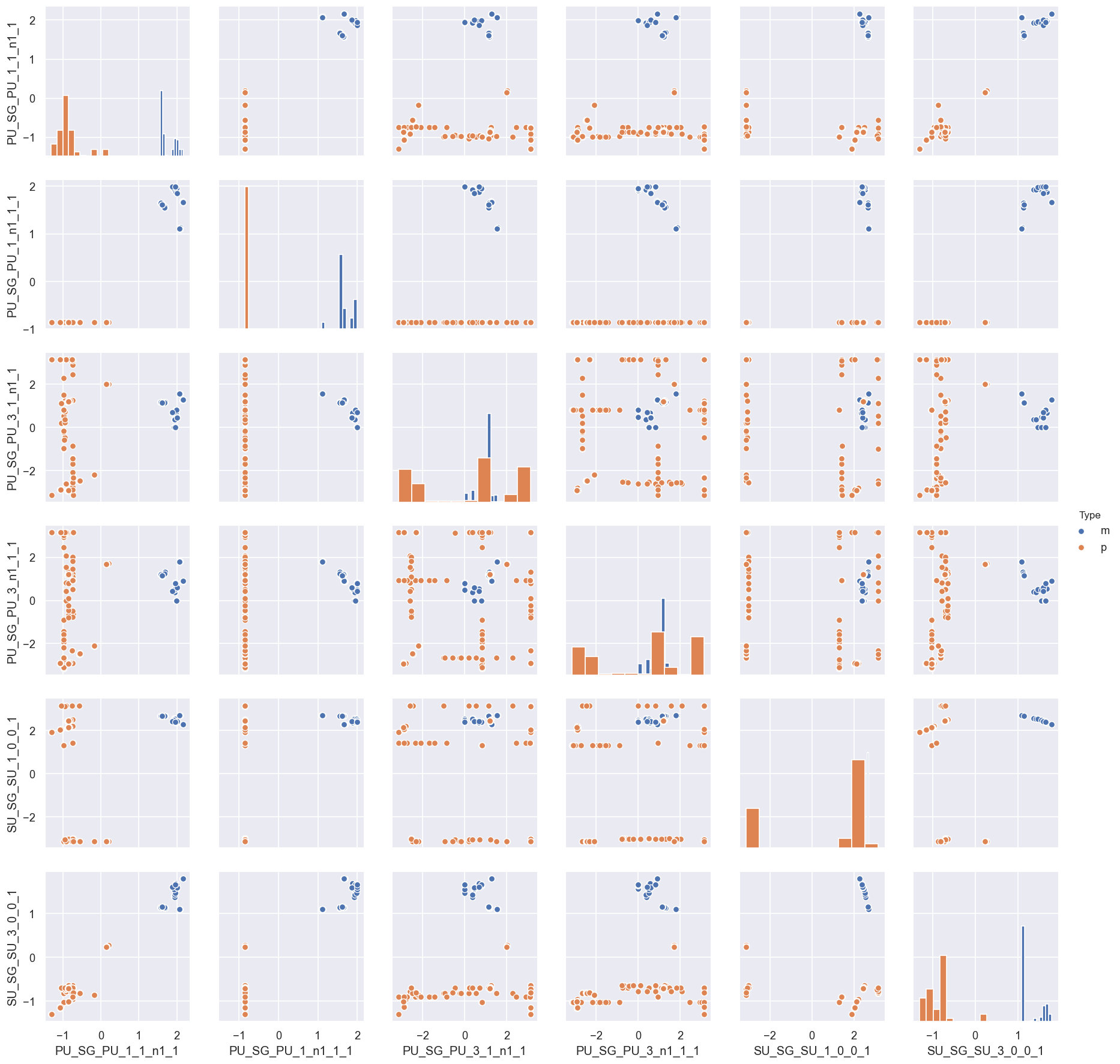
# For more control, standard catplot parameters can be passed.
# See https://seaborn.pydata.org/generated/seaborn.pairplot.html
# Plot with colour by Type and histograms on the diagonal
data.corrPlot(hue='Type', diag_kind='hist')
# Additional per-fit data can also be set for the hue mapping,
# e.g. plot with colour by redchi (to 6 dp) and histograms on the diagonal
# data.corrPlot(hue='redchi', hRound = 6, diag_kind='hist')
Mask not set for dataType = None.
*** Warning: found MultiIndex for DataFrame data.index - checkDims doesn't yet support Pandas MultiIndex.
<seaborn.axisgrid.PairGrid at 0x2051b21eeb8>
[13]:
# Tabulated output from the last plot can be found in self.data['plots']['<plotType>Data'], and the plot object in self.data['plots']['<plotType>Plot']
data.data['plots']['corrData']
[13]:
| Param | Type | redchiGroup | PU_SG_PU_1_1_n1_1 | PU_SG_PU_1_n1_1_1 | PU_SG_PU_3_1_n1_1 | PU_SG_PU_3_n1_1_1 | SU_SG_SU_1_0_0_1 | SU_SG_SU_3_0_0_1 |
|---|---|---|---|---|---|---|---|---|
| 0 | m | Q | 1.992972 | 1.921566 | 0.466055 | 0.000100 | 2.461439 | 1.556832 |
| 1 | p | Q | -0.861561 | -0.861041 | 3.141575 | 1.313656 | -3.032645 | -0.647618 |
| 2 | m | E | 1.609869 | 1.617583 | 1.141043 | 1.143667 | 2.652536 | 1.143790 |
| 3 | p | E | -0.857299 | -0.861041 | 1.199021 | 1.200058 | 2.437037 | -0.704019 |
| 4 | m | K | 1.932782 | 1.931857 | 0.355341 | 0.368418 | 2.533506 | 1.418030 |
| ... | ... | ... | ... | ... | ... | ... | ... | ... |
| 1117 | p | L | 0.145056 | -0.861041 | 2.001652 | 1.692756 | -3.141593 | 0.230230 |
| 1118 | m | N | 1.952031 | 1.992561 | 0.000100 | 0.805098 | 2.387993 | 1.651091 |
| 1119 | p | N | -0.739526 | -0.861041 | -1.434696 | 0.937920 | 1.420065 | -0.905355 |
| 1120 | m | E | 1.613212 | 1.614101 | 1.142782 | 1.142106 | 2.652523 | 1.143815 |
| 1121 | p | E | -0.862937 | -0.861041 | 1.195923 | 1.197572 | 2.434125 | -0.708249 |
1122 rows × 8 columns
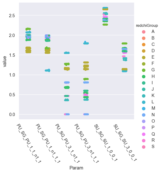
paramPlot()
For examining specific datatypes in more detail paramPlot() uses Seaborn’s catplot routine to generate scatter plots for a specified data type.
[14]:
# Plot all data, magnitudes
data.paramPlot(dataType='m')
Mask not set for dataType = None.
*** Warning: found MultiIndex for DataFrame data.index - checkDims doesn't yet support Pandas MultiIndex.
<seaborn.axisgrid.FacetGrid at 0x2051e7fa240>
[15]:
# Plot all data, phases
data.paramPlot(dataType='p')
Mask not set for dataType = None.
*** Warning: found MultiIndex for DataFrame data.index - checkDims doesn't yet support Pandas MultiIndex.
<seaborn.axisgrid.FacetGrid at 0x2051e9c09e8>
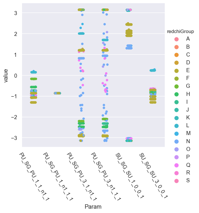
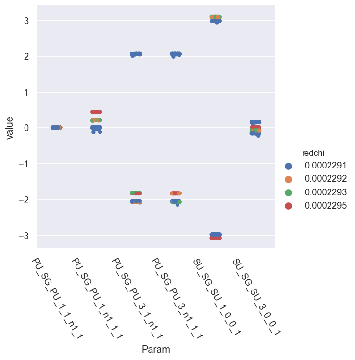
Here we can see that there are various sets of parameters which do, indeed, cluster by group (hence \(\chi^2\)) for the most part, although there is a full spread in some of the phase parameters. We can look more closely at this by selecting just the best group(s) and colour-coding by \(\chi^2\)…
[16]:
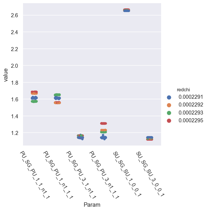
# Subselect on redchiGroup and colour by redchi value (note this automatically rounds to 7 dp, set hRound = N to control this)
data.paramPlot(dataType='m', sel = 'E', hue = 'redchi')
Mask not set for dataType = None.
<seaborn.axisgrid.FacetGrid at 0x2051eb04c50>
[17]:
# As above, but for phase data
data.paramPlot(dataType='p', sel = 'E', hue = 'redchi')
Mask not set for dataType = None.
<seaborn.axisgrid.FacetGrid at 0x2051fd0bdd8>
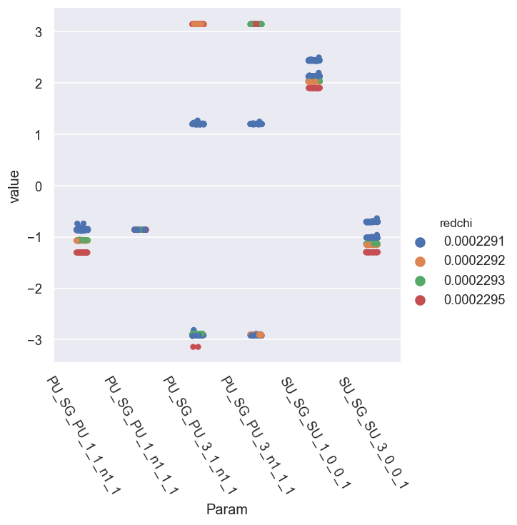
In this case, there are clear sub-groupings by \(\chi^2\). For the phases, these can potentially be cleaned up a bit by setting a reference phase & wrapping the values.
[18]:
# Tabulated output from the last plot can be found in self.data['plots']['<plotType>Data'], and the plot object in self.data['plots']['<plotType>Plot']
data.data['plots']['paramData']
[18]:
| Fit | Param | value | redchi | |
|---|---|---|---|---|
| 0 | 2 | PU_SG_PU_1_1_n1_1 | -0.857299 | 0.000229 |
| 1 | 8 | PU_SG_PU_1_1_n1_1 | -1.057287 | 0.000229 |
| 2 | 9 | PU_SG_PU_1_1_n1_1 | -1.303957 | 0.000229 |
| 3 | 11 | PU_SG_PU_1_1_n1_1 | -0.862917 | 0.000229 |
| 4 | 13 | PU_SG_PU_1_1_n1_1 | -0.863154 | 0.000229 |
| ... | ... | ... | ... | ... |
| 2089 | 984 | SU_SG_SU_3_0_0_1 | -0.702315 | 0.000229 |
| 2090 | 987 | SU_SG_SU_3_0_0_1 | -0.704560 | 0.000229 |
| 2091 | 988 | SU_SG_SU_3_0_0_1 | -1.015555 | 0.000229 |
| 2092 | 992 | SU_SG_SU_3_0_0_1 | -0.710594 | 0.000229 |
| 2093 | 997 | SU_SG_SU_3_0_0_1 | -0.708249 | 0.000229 |
2094 rows × 4 columns
[19]:
# Basic Holoviews support is also working, with a few additional plot options
# data.paramPlot(dataType='p', backend='hv')
data.paramPlot(dataType='p', backend='hv', hvType='violin') # Include violin KDE
Mask not set for dataType = None.
*** Warning: found MultiIndex for DataFrame data.index - checkDims doesn't yet support Pandas MultiIndex.
[20]:
# Single group with 'redchi' cmap
data.paramPlot(dataType='p', sel = 'E', hue = 'redchi', backend='hv', hvType='violin')
# data.paramPlot(dataType='p', sel = 'E', backend='hv') # NOTE: this currently doesn't work without Hue set to a numerical category.
Mask not set for dataType = None.
Phase shifts & corrections
To set the phases relative to a speific parameter, and wrap to a specified range, use the phaseCorrection() method. This defaults to using the first parameter as a reference phase, and wraps to \(-\pi:\pi\). The phase-corrected values are output to a new Type, ‘pc’.
[21]:
# Phase correction method
# This defaults to using the first parameter as a reference phase. The phase-corrected values are output to a new Type, 'pc'.
data.phaseCorrection()
Setting wide-form data self.[fits][dfWide] from self.[fits][dfLong] (as pivot table).
*** Warning: found MultiIndex for DataFrame data.index - checkDims doesn't yet support Pandas MultiIndex.
*** Warning: found MultiIndex for DataFrame data.index - checkDims doesn't yet support Pandas MultiIndex.
Index(es) = ['Fit', 'Type', 'redchiGroup'], cols = value
Set ref param = PU_SG_PU_1_1_n1_1
| Param | PU_SG_PU_1_1_n1_1 | PU_SG_PU_1_n1_1_1 | PU_SG_PU_3_1_n1_1 | PU_SG_PU_3_n1_1_1 | SU_SG_SU_1_0_0_1 | SU_SG_SU_3_0_0_1 | ||
|---|---|---|---|---|---|---|---|---|
| Fit | Type | redchiGroup | ||||||
| 1 | m | Q | 1.992972 | 1.921566 | 0.466055 | 0.000100 | 2.461439 | 1.556832 |
| p | Q | -0.861561 | -0.861041 | 3.141575 | 1.313656 | -3.032645 | -0.647618 | |
| pc | Q | 0.000000 | 0.000519 | -2.280049 | 2.175216 | -2.171084 | 0.213943 | |
| 2 | m | E | 1.609869 | 1.617583 | 1.141043 | 1.143667 | 2.652536 | 1.143790 |
| p | E | -0.857299 | -0.861041 | 1.199021 | 1.200058 | 2.437037 | -0.704019 | |
| ... | ... | ... | ... | ... | ... | ... | ... | ... |
| 996 | p | N | -0.739526 | -0.861041 | -1.434696 | 0.937920 | 1.420065 | -0.905355 |
| pc | N | 0.000000 | -0.121515 | -0.695170 | 1.677446 | 2.159591 | -0.165829 | |
| 997 | m | E | 1.613212 | 1.614101 | 1.142782 | 1.142106 | 2.652523 | 1.143815 |
| p | E | -0.862937 | -0.861041 | 1.195923 | 1.197572 | 2.434125 | -0.708249 | |
| pc | E | 0.000000 | 0.001896 | 2.058860 | 2.060509 | -2.986124 | 0.154688 |
1683 rows × 6 columns
We can replot the best fits for the phase-corrected case… this looks slightly cleaner, but still shows some +/- pairs and spread in retrieved values.
[22]:
data.paramPlot(dataType='pc', sel = 'E', hue = 'redchi')
Mask not set for dataType = None.
<seaborn.axisgrid.FacetGrid at 0x2051de4d438>
[23]:
# data.data[1]['results'] #.keys() #['fits']['dfRef'] #.keys()
Selecting & testing candidate parameter sets
After reviewing a batch of results (parameter sets), the best result(s) need more careful investigation…
[24]:
# Set new classifiers for small range
data.classifyFits(bins = [2.29e-4, 2.3e-4,20])
| success | chisqr | redchi | Min | Max | ||||||||||
|---|---|---|---|---|---|---|---|---|---|---|---|---|---|---|
| count | unique | top | freq | count | unique | top | freq | count | unique | top | freq | |||
| redchiGroup | ||||||||||||||
| A | 0 | 0 | NaN | NaN | 0 | 0 | NaN | NaN | 0 | 0 | NaN | NaN | 0.000229 | 0.000229 |
| B | 0 | 0 | NaN | NaN | 0 | 0 | NaN | NaN | 0 | 0 | NaN | NaN | 0.000229 | 0.000229 |
| C | 203 | 1 | True | 203 | 203 | 203 | 0.0421575 | 1 | 203 | 203 | 0.000229117 | 1 | 0.000229 | 0.000229 |
| D | 0 | 0 | NaN | NaN | 0 | 0 | NaN | NaN | 0 | 0 | NaN | NaN | 0.000229 | 0.000229 |
| E | 44 | 1 | True | 44 | 44 | 44 | 0.0421805 | 1 | 44 | 44 | 0.000229242 | 1 | 0.000229 | 0.000229 |
| F | 0 | 0 | NaN | NaN | 0 | 0 | NaN | NaN | 0 | 0 | NaN | NaN | 0.000229 | 0.000229 |
| G | 55 | 1 | True | 55 | 55 | 55 | 0.0421963 | 1 | 55 | 55 | 0.000229328 | 1 | 0.000229 | 0.000229 |
| H | 0 | 0 | NaN | NaN | 0 | 0 | NaN | NaN | 0 | 0 | NaN | NaN | 0.000229 | 0.000229 |
| I | 0 | 0 | NaN | NaN | 0 | 0 | NaN | NaN | 0 | 0 | NaN | NaN | 0.000229 | 0.000229 |
| J | 0 | 0 | NaN | NaN | 0 | 0 | NaN | NaN | 0 | 0 | NaN | NaN | 0.000229 | 0.000230 |
| K | 47 | 1 | True | 47 | 47 | 47 | 0.0422356 | 1 | 47 | 47 | 0.000229542 | 1 | 0.000230 | 0.000230 |
| L | 0 | 0 | NaN | NaN | 0 | 0 | NaN | NaN | 0 | 0 | NaN | NaN | 0.000230 | 0.000230 |
| M | 0 | 0 | NaN | NaN | 0 | 0 | NaN | NaN | 0 | 0 | NaN | NaN | 0.000230 | 0.000230 |
| N | 0 | 0 | NaN | NaN | 0 | 0 | NaN | NaN | 0 | 0 | NaN | NaN | 0.000230 | 0.000230 |
| O | 0 | 0 | NaN | NaN | 0 | 0 | NaN | NaN | 0 | 0 | NaN | NaN | 0.000230 | 0.000230 |
| P | 0 | 0 | NaN | NaN | 0 | 0 | NaN | NaN | 0 | 0 | NaN | NaN | 0.000230 | 0.000230 |
| Q | 0 | 0 | NaN | NaN | 0 | 0 | NaN | NaN | 0 | 0 | NaN | NaN | 0.000230 | 0.000230 |
| R | 0 | 0 | NaN | NaN | 0 | 0 | NaN | NaN | 0 | 0 | NaN | NaN | 0.000230 | 0.000230 |
| S | 0 | 0 | NaN | NaN | 0 | 0 | NaN | NaN | 0 | 0 | NaN | NaN | 0.000230 | 0.000230 |
Setting wide-form data self.[fits][dfWide] from self.[fits][dfLong] (as pivot table).
*** Warning: found MultiIndex for DataFrame data.index - checkDims doesn't yet support Pandas MultiIndex.
*** Warning: found MultiIndex for DataFrame data.index - checkDims doesn't yet support Pandas MultiIndex.
Index(es) = ['Fit', 'Type', 'redchiGroup'], cols = value
Set redchiGroup for data frame dfLong.
Set redchiGroup for data frame AFpdLong.
Couldn't set redchiGroup for data frame mask. Error <class 'KeyError'>: ('dType',).
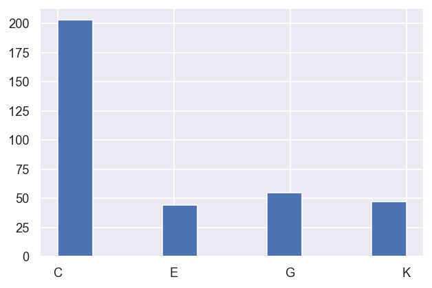
Drill down into the best (lowest \(\chi^2\)) grouping ‘C’…
[25]:
# Note hRound (== decimal places) specified to avoid collapsing colour-mapping to a single value.
data.paramPlot(dataType='m', sel = 'C', hue = 'redchi', backend='hv', hvType='box', hRound = 9)
Mask not set for dataType = None.
[26]:
data.paramPlot(dataType='p', sel = 'C', hue = 'redchi', backend='hv', hRound = 9) # Plot with redchi cmap
# data.paramPlot(dataType='pc', sel = 'C', hue = 'Fit', backend='hv', hRound = 9) # Plot with Fit # cmap
Mask not set for dataType = None.
In this case, the results look consistent for both magnitudes and phases (with +/- pairs evident in the latter case). We can look more carefully at any correlations here with corrPlot() with subselections (TODO: make this cleaner!).
[27]:
# corrPlot() with subselections (two levels)
# NOTE: with hue mapping for a continuous range this can be quite slow (minutes).
data.corrPlot(dataType = 'C', level = 'redchiGroup', sel = 'p', selLevel = 'Type', hue = 'redchi') #, diag_kind = 'scatter')
# For a faster plot either skip hue mapping and force diag to scatter (otherwise KDE generation can be slow)
# data.corrPlot(dataType = 'C', level = 'redchiGroup', sel = 'p', selLevel = 'Type', diag_kind = 'scatter')
Mask not set for dataType = None.
<seaborn.axisgrid.PairGrid at 0x2051ebd7438>
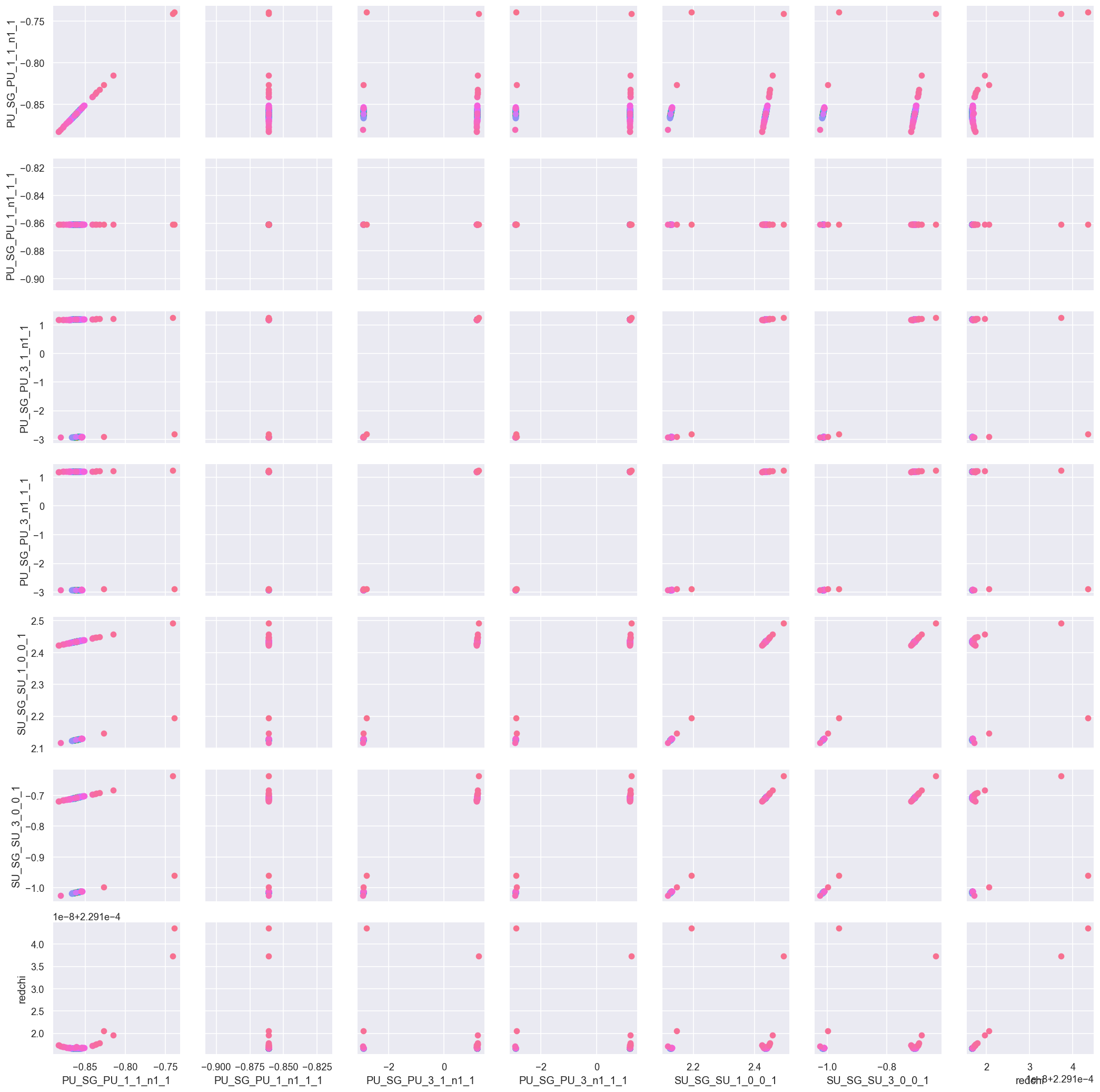
In this case there appears to be a direct correlation between +/- phase pairs over all parameters - for example, the third row (PU_SG_PU_3_1_n1_1) appears to show only +ve results sets or -ve results sets. This is expected if the dataset is not sensitive to the sign of the phases, and means that the phases are essentially defined modulo(\(\pi\)).
Again, the phase-corrected values can also be defined & visualised to check this, and can also be mapped to the range \(0:\pi\) by setting absFlag=True.
[28]:
data.phaseCorrection(absFlag=True) # NOTE - need to rerun phaseCorrection after classification
# data.phaseCorrection()
data.paramPlot(dataType='pc', sel = 'C', hue = 'redchi', backend='hv', hRound = 9)
Setting wide-form data self.[fits][dfWide] from self.[fits][dfLong] (as pivot table).
*** Warning: found MultiIndex for DataFrame data.index - checkDims doesn't yet support Pandas MultiIndex.
*** Warning: found MultiIndex for DataFrame data.index - checkDims doesn't yet support Pandas MultiIndex.
Index(es) = ['Fit', 'Type', 'redchiGroup'], cols = value
Set ref param = PU_SG_PU_1_1_n1_1
| Param | PU_SG_PU_1_1_n1_1 | PU_SG_PU_1_n1_1_1 | PU_SG_PU_3_1_n1_1 | PU_SG_PU_3_n1_1_1 | SU_SG_SU_1_0_0_1 | SU_SG_SU_3_0_0_1 | ||
|---|---|---|---|---|---|---|---|---|
| Fit | Type | redchiGroup | ||||||
| 2 | m | C | 1.609869 | 1.617583 | 1.141043 | 1.143667 | 2.652536 | 1.143790 |
| p | C | -0.857299 | -0.861041 | 1.199021 | 1.200058 | 2.437037 | -0.704019 | |
| pc | C | 0.000000 | 0.003742 | 2.056320 | 2.057357 | 2.988849 | 0.153280 | |
| 8 | m | G | 1.569258 | 1.654651 | 1.166865 | 1.207240 | 2.659540 | 1.129703 |
| p | G | -1.057287 | -0.861041 | -2.876167 | 3.141593 | 2.040967 | -1.129251 | |
| ... | ... | ... | ... | ... | ... | ... | ... | ... |
| 992 | p | C | -0.867768 | -0.861041 | 1.193419 | 1.195135 | 2.431628 | -0.710594 |
| pc | C | 0.000000 | 0.006727 | 2.061187 | 2.062903 | 2.983790 | 0.157174 | |
| 997 | m | C | 1.613212 | 1.614101 | 1.142782 | 1.142106 | 2.652523 | 1.143815 |
| p | C | -0.862937 | -0.861041 | 1.195923 | 1.197572 | 2.434125 | -0.708249 | |
| pc | C | 0.000000 | 0.001896 | 2.058860 | 2.060509 | 2.986124 | 0.154688 |
1047 rows × 6 columns
Mask not set for dataType = None.
[29]:
# corrPlot() with subselections (two levels)
# NOTE: with hue mapping for a continuous range this can be quite slow (minutes).
data.corrPlot(dataType = 'C', level = 'redchiGroup', sel = 'pc', selLevel = 'Type', hue = 'redchi') # Check pair correlations including redchi
# data.corrPlot(dataType = 'C', level = 'redchiGroup', sel = 'pc', selLevel = 'Type', hue = 'Fit') # Check pair correlations including Fit #
Mask not set for dataType = None.
<seaborn.axisgrid.PairGrid at 0x2052b4c42b0>
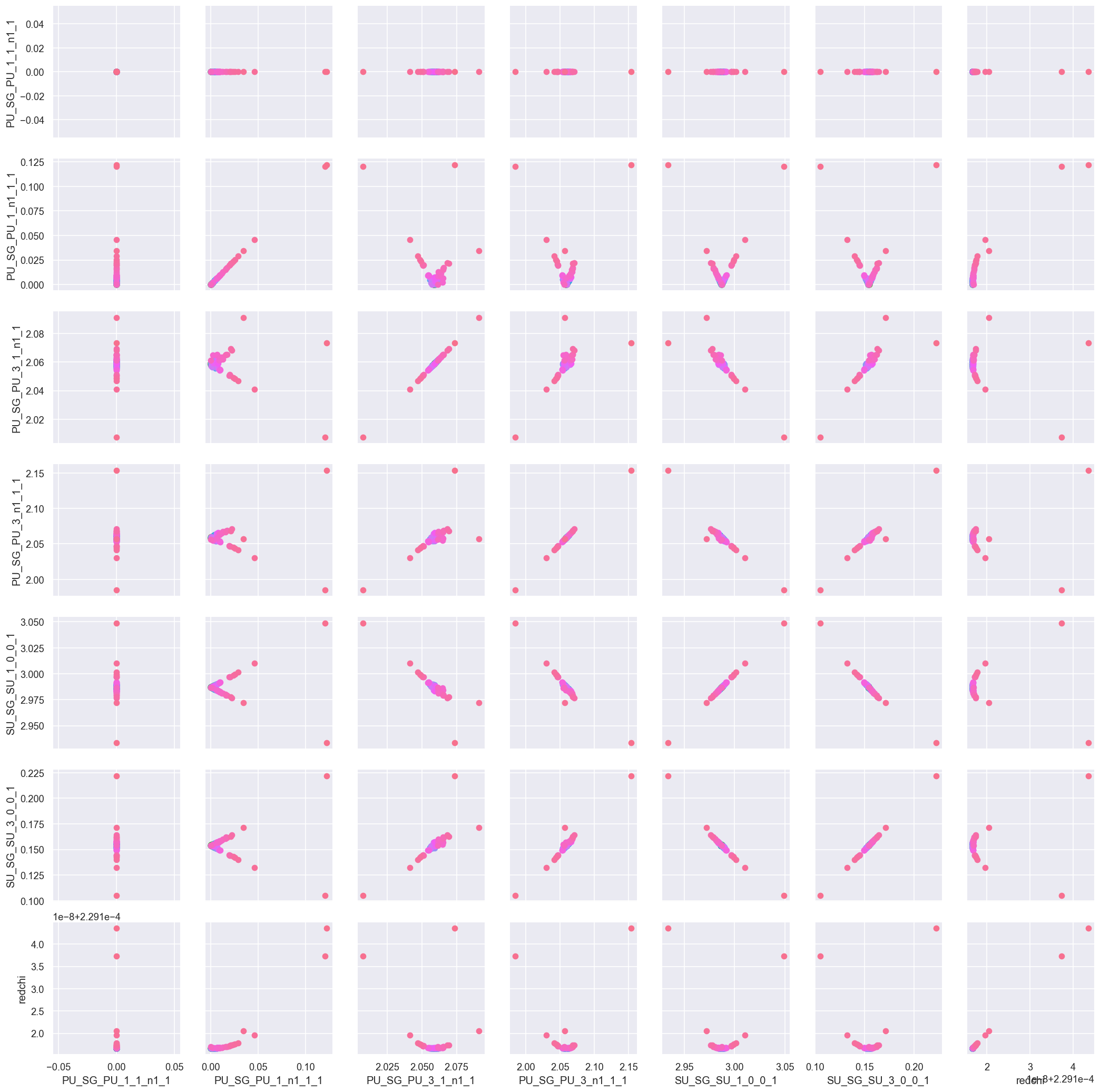
Here a few things are clearer - in particular the relative phases seem to be well-behaved, with a fairly small scatter, and the (1D) minima of the fitting hyperspace are visible in the \(\chi^2\) plots (bottom row).
Best values and statistics
To get a final parameter set and associated statistics, based on a subset of the fit results, the paramsReport() method is available. In this case, it will provide summary statistics corresponding to the corrPlot() above.
[30]:
# Get parameter statistics.
# Specify subselection criteria with a dictionary of selectors (currently uses index values only)
# TODO: more general selection & groupings here.
data.paramsReport(inds = {'redchiGroup':'C'})
Mask not set for dataType = None.
Set parameter stats to self.paramsSummary.
| Type | m | p | pc | |
|---|---|---|---|---|
| Param | Agg | |||
| PU_SG_PU_1_1_n1_1 | min | 1.605239e+00 | -0.883176 | 0.000000 |
| mean | 1.613850e+00 | -0.859382 | 0.000000 | |
| median | 1.613657e+00 | -0.860940 | 0.000000 | |
| max | 1.625738e+00 | -0.738983 | 0.000000 | |
| std | 2.084992e-03 | 0.014059 | 0.000000 | |
| var | 4.347190e-06 | 0.000198 | 0.000000 | |
| PU_SG_PU_1_n1_1_1 | min | 1.601543e+00 | -0.861041 | 0.000019 |
| mean | 1.613570e+00 | -0.861041 | 0.005372 | |
| median | 1.613690e+00 | -0.861041 | 0.002132 | |
| max | 1.627827e+00 | -0.861041 | 0.122059 | |
| std | 2.202383e-03 | 0.000000 | 0.013093 | |
| var | 4.850490e-06 | 0.000000 | 0.000171 | |
| PU_SG_PU_3_1_n1_1 | min | 1.124479e+00 | -2.931328 | 2.007461 |
| mean | 1.142652e+00 | 0.144138 | 2.058870 | |
| median | 1.142526e+00 | 1.196919 | 2.058890 | |
| max | 1.174468e+00 | 1.266499 | 2.091134 | |
| std | 3.045999e-03 | 1.800711 | 0.005289 | |
| var | 9.278107e-06 | 3.242561 | 0.000028 | |
| PU_SG_PU_3_n1_1_1 | min | 1.124041e+00 | -2.927744 | 1.984783 |
| mean | 1.142349e+00 | 0.143498 | 2.058926 | |
| median | 1.142249e+00 | 1.196777 | 2.058825 | |
| max | 1.172665e+00 | 1.243822 | 2.154092 | |
| std | 3.032450e-03 | 1.801116 | 0.009501 | |
| var | 9.195751e-06 | 3.244017 | 0.000090 | |
| SU_SG_SU_1_0_0_1 | min | 2.652285e+00 | 2.116167 | 2.933528 |
| mean | 2.652524e+00 | 2.356759 | 2.986923 | |
| median | 2.652526e+00 | 2.434259 | 2.986913 | |
| max | 2.653001e+00 | 2.493262 | 3.048962 | |
| std | 4.240577e-05 | 0.134550 | 0.006770 | |
| var | 1.798250e-09 | 0.018104 | 0.000046 | |
| SU_SG_SU_3_0_0_1 | min | 1.142825e+00 | -1.025558 | 0.105030 |
| mean | 1.143807e+00 | -0.785126 | 0.154275 | |
| median | 1.143806e+00 | -0.708064 | 0.154106 | |
| max | 1.144052e+00 | -0.635932 | 0.222062 | |
| std | 7.751534e-05 | 0.134263 | 0.006839 | |
| var | 6.008628e-09 | 0.018027 | 0.000047 |
[31]:
# For more control, pass a list of aggregation functions
# These are passed to Pandas.agg(), a list of common functions can be found at https://pandas.pydata.org/docs/user_guide/basics.html#descriptive-statistics
data.paramsReport(inds = {'redchiGroup':'C'}, aggList = ['mean', 'std'])
Mask not set for dataType = None.
Set parameter stats to self.paramsSummary.
| Type | m | p | pc | |
|---|---|---|---|---|
| Param | Agg | |||
| PU_SG_PU_1_1_n1_1 | mean | 1.613850 | -0.859382 | 0.000000 |
| std | 0.002085 | 0.014059 | 0.000000 | |
| PU_SG_PU_1_n1_1_1 | mean | 1.613570 | -0.861041 | 0.005372 |
| std | 0.002202 | 0.000000 | 0.013093 | |
| PU_SG_PU_3_1_n1_1 | mean | 1.142652 | 0.144138 | 2.058870 |
| std | 0.003046 | 1.800711 | 0.005289 | |
| PU_SG_PU_3_n1_1_1 | mean | 1.142349 | 0.143498 | 2.058926 |
| std | 0.003032 | 1.801116 | 0.009501 | |
| SU_SG_SU_1_0_0_1 | mean | 2.652524 | 2.356759 | 2.986923 |
| std | 0.000042 | 0.134550 | 0.006770 | |
| SU_SG_SU_3_0_0_1 | mean | 1.143807 | -0.785126 | 0.154275 |
| std | 0.000078 | 0.134263 | 0.006839 |
Model results
For each fit, the model output (AF-\(\beta_{LM}\) parameter) can also be investigated…
Basic plotters
Basic per-fit outputs using wrapped ePSproc routines.
[32]:
# Plot selected results from per-fit datasets.
data.BLMfitPlot(keys = ['subset', 0, 50]) # This works, but need to add selectors? And control output.
Dataset: subset, AFBLM
Dataset: 0, AFBLM
Dataset: 50, AFBLM
[33]:
# Per-fit strip-chart style plotting (inc. all labelled dims) with lmPlot() wrapper.
# NOTE: self.lmPlotOpts will be set and is sticky. (As per epsproc-dev version 23/11/21)
# data.lmPlotFit(keys = ['subset', 0, 50])
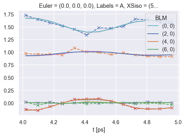
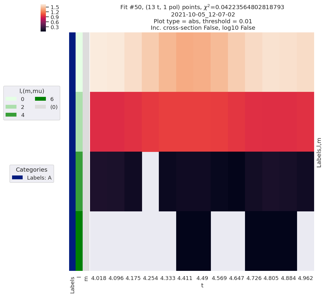
data.lmPlotFit(keys = [50]) #, xDim=['t'])
Plotting data (No filename), pType=a, thres=0.01, with Seaborn
D:\code\github\ePSproc\epsproc\_sns_matrixMod.py:282: PendingDeprecationWarning:
The label function will be deprecated in a future version. Use Tick.label1 instead.
fontsize = tick.label.get_size()
Fit set plotters
For large sets the BLMsetPlot() method implements Holoviews to allow for fit browsing and aggregations.
For manual examples with Seaborn (not yet wrapped), see https://pemtk.readthedocs.io/en/latest/fitting/PEMtk_analysis_demo_150621-tidy.html#Model-results
[34]:
# The default routine aggreagates over all fits (mean + std for spread) and stacks plots
# Set xDim to ensure consistent plotting
data.BLMsetPlot(xDim = 't')
[35]:
# Browse a set of fits interactively.
# Note this may be slow to render for large datasets (==minutes) if ref data is included.
# Get indexes for a group
inds = data.getFitInds(selectors = {'redchiGroup':'C'} )
# HV plot without aggregation - this will automatically Holomap other dims
data.BLMsetPlot(xDim = 't', sel = {'Fit':inds}, agg = False, ref = False)
Mask not set for dataType = None.
Comparison of parameters/matrix elements with inputs (if known)
For model data and testing the final parameter set(s) can be compared with the known inputs. This is facilitated by the paramsCompare() method. This compares the data in self.paramsSummary with self.params. If not set, the routine will attempt to set these from defaults (for input values this may be in self.data['fits']['dfRef'] or will be pulled from the matrix elements in self.data['subset']['matE']).
TODO: generalise the routine for comparison of arb pairs/sets of parameters.
[36]:
# Run with defaults.
# Note this will produce extra output if setting self.params, as in this example
data.paramsCompare()
self.params not set, setting ref values from self.data[subset]['matE'] without constraints.
Set 6 complex matrix elements to 12 fitting params, see self.params for details.
| name | value | initial value | min | max | vary |
|---|---|---|---|---|---|
| m_PU_SG_PU_1_n1_1_1 | 1.78461575 | 1.784615753610107 | 1.0000e-04 | 5.00000000 | True |
| m_PU_SG_PU_1_1_n1_1 | 1.78461575 | 1.784615753610107 | 1.0000e-04 | 5.00000000 | True |
| m_PU_SG_PU_3_n1_1_1 | 0.80290495 | 0.802904951323892 | 1.0000e-04 | 5.00000000 | True |
| m_PU_SG_PU_3_1_n1_1 | 0.80290495 | 0.802904951323892 | 1.0000e-04 | 5.00000000 | True |
| m_SU_SG_SU_1_0_0_1 | 2.68606212 | 2.686062120382649 | 1.0000e-04 | 5.00000000 | True |
| m_SU_SG_SU_3_0_0_1 | 1.10915311 | 1.109153108617096 | 1.0000e-04 | 5.00000000 | True |
| p_PU_SG_PU_1_n1_1_1 | -0.86104140 | -0.8610414024232179 | -3.14159265 | 3.14159265 | False |
| p_PU_SG_PU_1_1_n1_1 | -0.86104140 | -0.8610414024232179 | -3.14159265 | 3.14159265 | True |
| p_PU_SG_PU_3_n1_1_1 | -3.12044446 | -3.1204444620772467 | -3.14159265 | 3.14159265 | True |
| p_PU_SG_PU_3_1_n1_1 | -3.12044446 | -3.1204444620772467 | -3.14159265 | 3.14159265 | True |
| p_SU_SG_SU_1_0_0_1 | 2.61122920 | 2.611229196458127 | -3.14159265 | 3.14159265 | True |
| p_SU_SG_SU_3_0_0_1 | -0.07867828 | -0.07867827542158025 | -3.14159265 | 3.14159265 | True |
Setting wide-form data self.[fits][dfWide] from self.[fits][dfLong] (as pivot table).
*** Warning: found MultiIndex for DataFrame data.index - checkDims doesn't yet support Pandas MultiIndex.
*** Warning: found MultiIndex for DataFrame data.index - checkDims doesn't yet support Pandas MultiIndex.
Index(es) = ['Fit', 'Type'], cols = value
Set ref param = PU_SG_PU_1_1_n1_1
| Param | PU_SG_PU_1_1_n1_1 | PU_SG_PU_1_n1_1_1 | PU_SG_PU_3_1_n1_1 | PU_SG_PU_3_n1_1_1 | SU_SG_SU_1_0_0_1 | SU_SG_SU_3_0_0_1 | |
|---|---|---|---|---|---|---|---|
| Fit | Type | ||||||
| ref | m | 1.784616 | 1.784616 | 0.802905 | 0.802905 | 2.686062 | 1.109153 |
| p | -0.861041 | -0.861041 | -3.120444 | -3.120444 | 2.611229 | -0.078678 | |
| pc | 0.000000 | 0.000000 | -2.259403 | -2.259403 | -2.810915 | 0.782363 |
C:\Users\femtolab\.conda\envs\ePSdev\lib\site-packages\IPython\core\interactiveshell.py:2886: PerformanceWarning: indexing past lexsort depth may impact performance.
return runner(coro)
Set parameter comparison to self.paramsSummaryComp.
| Param | PU_SG_PU_1_1_n1_1 | PU_SG_PU_1_n1_1_1 | PU_SG_PU_3_1_n1_1 | PU_SG_PU_3_n1_1_1 | SU_SG_SU_1_0_0_1 | SU_SG_SU_3_0_0_1 | ||
|---|---|---|---|---|---|---|---|---|
| Type | Source | dType | ||||||
| m | mean | num | 1.613850 | 1.613570e+00 | 1.142652 | 1.142349 | 2.652524 | 1.143807 |
| ref | num | 1.784616 | 1.784616e+00 | 0.802905 | 0.802905 | 2.686062 | 1.109153 | |
| diff | % | 10.581260 | 1.060047e+01 | 29.733209 | 29.714546 | 1.264393 | 3.029722 | |
| num | -0.170766 | -1.710460e-01 | 0.339747 | 0.339444 | -0.033538 | 0.034654 | ||
| std | % | 0.129194 | 1.364913e-01 | 0.266573 | 0.265457 | 0.001599 | 0.006777 | |
| num | 0.002085 | 2.202383e-03 | 0.003046 | 0.003032 | 0.000042 | 0.000078 | ||
| diff/std | % | 8190.232468 | 7.766406e+03 | 11153.883911 | 11193.713369 | 79089.050126 | 44706.225465 | |
| p | mean | num | -0.859382 | -8.610414e-01 | 0.144138 | 0.143498 | 2.356759 | -0.785126 |
| ref | num | -0.861041 | -8.610414e-01 | -3.120444 | -3.120444 | 2.611229 | -0.078678 | |
| diff | % | 0.193090 | 4.512885e-13 | 2264.893304 | 2274.558140 | 10.797481 | 89.978902 | |
| num | 0.001659 | 3.885781e-15 | 3.264583 | 3.263942 | -0.254471 | -0.706448 | ||
| std | % | 1.635940 | 0.000000e+00 | 1249.292494 | 1255.151491 | 5.709133 | 17.100819 | |
| num | 0.014059 | 0.000000e+00 | 1.800711 | 1.801116 | 0.134550 | 0.134263 | ||
| diff/std | % | 11.802998 | inf | 181.294078 | 181.217818 | 189.126456 | 526.167201 | |
| pc | mean | num | 0.000000 | 5.372290e-03 | 2.058870 | 2.058926 | 2.986923 | 0.154275 |
| ref | num | 0.000000 | 0.000000e+00 | -2.259403 | -2.259403 | -2.810915 | 0.782363 | |
| diff | % | NaN | 1.000000e+02 | 209.739951 | 209.736965 | 194.107385 | 407.123575 | |
| num | 0.000000 | 5.372290e-03 | 4.318273 | 4.318329 | 5.797837 | -0.628088 | ||
| std | % | NaN | 2.437070e+02 | 0.256878 | 0.461470 | 0.226641 | 4.433055 | |
| num | 0.000000 | 1.309265e-02 | 0.005289 | 0.009501 | 0.006770 | 0.006839 | ||
| diff/std | % | NaN | 4.103288e+01 | 81649.662014 | 45449.762175 | 85645.382379 | 9183.815020 |
[37]:
# With abs phaseCorrection flag set
data.paramsCompare(phaseCorrParams={'absFlag':True})
Setting wide-form data self.[fits][dfWide] from self.[fits][dfLong] (as pivot table).
*** Warning: found MultiIndex for DataFrame data.index - checkDims doesn't yet support Pandas MultiIndex.
*** Warning: found MultiIndex for DataFrame data.index - checkDims doesn't yet support Pandas MultiIndex.
Index(es) = ['Fit', 'Type'], cols = value
Set ref param = PU_SG_PU_1_1_n1_1
| Param | PU_SG_PU_1_1_n1_1 | PU_SG_PU_1_n1_1_1 | PU_SG_PU_3_1_n1_1 | PU_SG_PU_3_n1_1_1 | SU_SG_SU_1_0_0_1 | SU_SG_SU_3_0_0_1 | |
|---|---|---|---|---|---|---|---|
| Fit | Type | ||||||
| ref | m | 1.784616 | 1.784616 | 0.802905 | 0.802905 | 2.686062 | 1.109153 |
| p | -0.861041 | -0.861041 | -3.120444 | -3.120444 | 2.611229 | -0.078678 | |
| pc | 0.000000 | 0.000000 | 2.259403 | 2.259403 | 2.810915 | 0.782363 |
C:\Users\femtolab\.conda\envs\ePSdev\lib\site-packages\IPython\core\interactiveshell.py:2886: PerformanceWarning: indexing past lexsort depth may impact performance.
return runner(coro)
Set parameter comparison to self.paramsSummaryComp.
| Param | PU_SG_PU_1_1_n1_1 | PU_SG_PU_1_n1_1_1 | PU_SG_PU_3_1_n1_1 | PU_SG_PU_3_n1_1_1 | SU_SG_SU_1_0_0_1 | SU_SG_SU_3_0_0_1 | ||
|---|---|---|---|---|---|---|---|---|
| Type | Source | dType | ||||||
| m | mean | num | 1.613850 | 1.613570e+00 | 1.142652 | 1.142349 | 2.652524 | 1.143807 |
| ref | num | 1.784616 | 1.784616e+00 | 0.802905 | 0.802905 | 2.686062 | 1.109153 | |
| diff | % | 10.581260 | 1.060047e+01 | 29.733209 | 29.714546 | 1.264393 | 3.029722 | |
| num | -0.170766 | -1.710460e-01 | 0.339747 | 0.339444 | -0.033538 | 0.034654 | ||
| std | % | 0.129194 | 1.364913e-01 | 0.266573 | 0.265457 | 0.001599 | 0.006777 | |
| num | 0.002085 | 2.202383e-03 | 0.003046 | 0.003032 | 0.000042 | 0.000078 | ||
| diff/std | % | 8190.232468 | 7.766406e+03 | 11153.883911 | 11193.713369 | 79089.050126 | 44706.225465 | |
| p | mean | num | -0.859382 | -8.610414e-01 | 0.144138 | 0.143498 | 2.356759 | -0.785126 |
| ref | num | -0.861041 | -8.610414e-01 | -3.120444 | -3.120444 | 2.611229 | -0.078678 | |
| diff | % | 0.193090 | 4.512885e-13 | 2264.893304 | 2274.558140 | 10.797481 | 89.978902 | |
| num | 0.001659 | 3.885781e-15 | 3.264583 | 3.263942 | -0.254471 | -0.706448 | ||
| std | % | 1.635940 | 0.000000e+00 | 1249.292494 | 1255.151491 | 5.709133 | 17.100819 | |
| num | 0.014059 | 0.000000e+00 | 1.800711 | 1.801116 | 0.134550 | 0.134263 | ||
| diff/std | % | 11.802998 | inf | 181.294078 | 181.217818 | 189.126456 | 526.167201 | |
| pc | mean | num | 0.000000 | 5.372290e-03 | 2.058870 | 2.058926 | 2.986923 | 0.154275 |
| ref | num | 0.000000 | 0.000000e+00 | 2.259403 | 2.259403 | 2.810915 | 0.782363 | |
| diff | % | NaN | 1.000000e+02 | 9.739951 | 9.736965 | 5.892615 | 407.123575 | |
| num | 0.000000 | 5.372290e-03 | -0.200533 | -0.200477 | 0.176008 | -0.628088 | ||
| std | % | NaN | 2.437070e+02 | 0.256878 | 0.461470 | 0.226641 | 4.433055 | |
| num | 0.000000 | 1.309265e-02 | 0.005289 | 0.009501 | 0.006770 | 0.006839 | ||
| diff/std | % | NaN | 4.103288e+01 | 3791.665217 | 2109.989164 | 2599.979908 | 9183.815020 |
In this particular case a few points of note:
The final results are generally quite close to the inputs. (In this case, the input dataset had reference data had ~10% random noise added, and the 1st phase was fixed as a reference during fitting; all other parameters were free.)
The absolute phase values appear to be quite far off in some cases, but the phase corrected values typically look quite good; this is consistent with a lack of sensitivity in the test dataset to the sign of the phases (as discussed elsewhere), but the remapped phases (\(0:\pi\)) are precise.
The differences between the data and reference values are much larger than the standard deviation of the fits. This is indicative of a good (==close/singular) batch of fits, but reveals that the results obtained are not perfect - as expected for noisey data. Adding more data-points to the fit, and/or using higher fidelity data would help in this case (and will be explored elsewhere in future).
Colour coding and further analysis may help with interpretation, see below for a quick demo.
[84]:
# Try checking full DF, rather than subset/slice - WITH ADDTIONS
# See, e.g., https://stackoverflow.com/questions/50220200/conditional-styling-in-pandas-using-other-columns
# Basically, set mask then styles in new dataframe.
import pandas as pd
idx = pd.IndexSlice
# This works for %/abs pairs
# Groupby to set for type subsets?
# Code from https://stackoverflow.com/questions/50220200/conditional-styling-in-pandas-using-other-columns
def select_pairs(x, props = '', bg = ''):
#compare columns
mask = idx[x.loc[idx[:,:,'%'],:] > 50] .droplevel('dType')
# mask = idx[data.paramsSummaryComp.loc[idx[:,:,'%'],:] > 50]
# mask = idx[x.loc[idx[:,:,'%']] > 50] # Select and drop - only works in pd >v1.2?
#DataFrame with same index and columns names as original filled empty strings
df1 = pd.DataFrame(bg, index=x.index, columns=x.columns)
#modify values of df1 column by boolean mask
# df1.where(mask, props, inplace = True)
df1.where(~(mask.reindex_like(x).fillna(False)), props, inplace = True)
return df1
# dfT.style.apply(highlight_cols, props='color:white;background-color:darkblue', axis=None) # OK
# data.paramsSummaryComp.style.apply(select_pairs, props='color:white;background-color:darkblue', axis=None) # OK
data.paramsSummaryComp.style.apply(select_pairs, props='background-color:orange',axis=None) # OK
[84]:
| Param | PU_SG_PU_1_1_n1_1 | PU_SG_PU_1_n1_1_1 | PU_SG_PU_3_1_n1_1 | PU_SG_PU_3_n1_1_1 | SU_SG_SU_1_0_0_1 | SU_SG_SU_3_0_0_1 | ||
|---|---|---|---|---|---|---|---|---|
| Type | Source | dType | ||||||
| m | mean | num | 1.613850 | 1.613570 | 1.142652 | 1.142349 | 2.652524 | 1.143807 |
| ref | num | 1.784616 | 1.784616 | 0.802905 | 0.802905 | 2.686062 | 1.109153 | |
| diff | % | 10.581260 | 10.600471 | 29.733209 | 29.714546 | 1.264393 | 3.029722 | |
| num | -0.170766 | -0.171046 | 0.339747 | 0.339444 | -0.033538 | 0.034654 | ||
| std | % | 0.129194 | 0.136491 | 0.266573 | 0.265457 | 0.001599 | 0.006777 | |
| num | 0.002085 | 0.002202 | 0.003046 | 0.003032 | 0.000042 | 0.000078 | ||
| diff/std | % | 8190.232468 | 7766.405823 | 11153.883911 | 11193.713369 | 79089.050126 | 44706.225465 | |
| p | mean | num | -0.859382 | -0.861041 | 0.144138 | 0.143498 | 2.356759 | -0.785126 |
| ref | num | -0.861041 | -0.861041 | -3.120444 | -3.120444 | 2.611229 | -0.078678 | |
| diff | % | 0.193090 | 0.000000 | 2264.893304 | 2274.558140 | 10.797481 | 89.978902 | |
| num | 0.001659 | 0.000000 | 3.264583 | 3.263942 | -0.254471 | -0.706448 | ||
| std | % | 1.635940 | 0.000000 | 1249.292494 | 1255.151491 | 5.709133 | 17.100819 | |
| num | 0.014059 | 0.000000 | 1.800711 | 1.801116 | 0.134550 | 0.134263 | ||
| diff/std | % | 11.802998 | inf | 181.294078 | 181.217818 | 189.126456 | 526.167201 | |
| pc | mean | num | 0.000000 | 0.005372 | 2.058870 | 2.058926 | 2.986923 | 0.154275 |
| ref | num | 0.000000 | 0.000000 | 2.259403 | 2.259403 | 2.810915 | 0.782363 | |
| diff | % | nan | 100.000000 | 9.739951 | 9.736965 | 5.892615 | 407.123575 | |
| num | 0.000000 | 0.005372 | -0.200533 | -0.200477 | 0.176008 | -0.628088 | ||
| std | % | nan | 243.707016 | 0.256878 | 0.461470 | 0.226641 | 4.433055 | |
| num | 0.000000 | 0.013093 | 0.005289 | 0.009501 | 0.006770 | 0.006839 | ||
| diff/std | % | nan | 41.032877 | 3791.665217 | 2109.989164 | 2599.979908 | 9183.815020 |
Versions
[39]:
import scooby
scooby.Report(additional=['epsproc', 'pemtk', 'xarray', 'jupyter'])
[39]:
| Tue Dec 07 10:44:58 2021 Eastern Standard Time | |||||
| OS | Windows | CPU(s) | 32 | Machine | AMD64 |
| Architecture | 64bit | RAM | 63.9 GB | Environment | Jupyter |
| Python 3.7.3 (default, Apr 24 2019, 15:29:51) [MSC v.1915 64 bit (AMD64)] | |||||
| epsproc | 1.3.1-dev | pemtk | 0.0.1 | xarray | 0.15.0 |
| jupyter | Version unknown | numpy | 1.19.2 | scipy | 1.3.0 |
| IPython | 7.12.0 | matplotlib | 3.3.1 | scooby | 0.5.6 |
| Intel(R) Math Kernel Library Version 2020.0.0 Product Build 20191125 for Intel(R) 64 architecture applications | |||||
[85]:
# Check current Git commit for local pemtk version
!git -C {Path(pemtk.__file__).parent} branch
!git -C {Path(pemtk.__file__).parent} log --format="%H" -n 1
* master
C:\Users\femtolab\.conda\envs\ePSdev\lib\site-packages\IPython\utils\_process_win32.py:131: ResourceWarning: unclosed file <_io.BufferedWriter name=8>
return process_handler(cmd, _system_body)
C:\Users\femtolab\.conda\envs\ePSdev\lib\site-packages\IPython\utils\_process_win32.py:131: ResourceWarning: unclosed file <_io.BufferedReader name=9>
return process_handler(cmd, _system_body)
C:\Users\femtolab\.conda\envs\ePSdev\lib\site-packages\IPython\utils\_process_win32.py:131: ResourceWarning: unclosed file <_io.BufferedReader name=10>
return process_handler(cmd, _system_body)
4d97c2d50d362168fd720c8c357b0f6e1eb66c3f
[86]:
# Check current remote commits
!git ls-remote --heads git://github.com/phockett/pemtk
# !git ls-remote --heads git://github.com/phockett/epsman
4d97c2d50d362168fd720c8c357b0f6e1eb66c3f refs/heads/master
[87]:
# Check current Git commit for local ePSproc version
import epsproc as ep
!git -C {Path(ep.__file__).parent} branch
!git -C {Path(ep.__file__).parent} log --format="%H" -n 1
* dev
master
numba-tests
5bfa0c6c47ed5f23eff65a290624ffff4e9c5924
[88]:
# Check current remote commits
!git ls-remote --heads git://github.com/phockett/ePSproc
# !git ls-remote --heads git://github.com/phockett/epsman
8fb518c63bfb4edc49ef994808f1c18fb68ff0c3 refs/heads/dependabot/pip/notes/envs/envs-versioned/pip-21.1
5bfa0c6c47ed5f23eff65a290624ffff4e9c5924 refs/heads/dev
5278f0389878f6e7e5eb9b0c013ff3594c70938f refs/heads/master
69cd89ce5bc0ad6d465a4bd8df6fba15d3fd1aee refs/heads/numba-tests
ea30878c842f09d525fbf39fa269fa2302a13b57 refs/heads/revert-9-master
[ ]: