Symmetrized harmonics demo

23/03/22

Changed coeffs to dict. self.coeffs[formats] now holds coeffs for formats libmsym, SH, DF and XR.
Added ePSproc data types interface.
Fixed plotXlm() for older versions of pySHtools (tested v4.5, current v4.9).
- Titles now OK.
- Colourbars not working in older versions?

16/03/22

Implemented in symHarm module as of b9d1e982.
Full API details in the docs.
Basic demo below.

Definitions

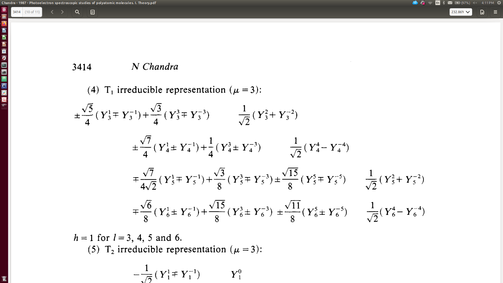
Symmetrized (or generalised) harmonics, which essentially provide correctly symmetrized expansions of spherical harmonics ($Y_{lm}$) functions for a given irreducible representation, $\Gamma$, can be defined by linear combinations of spherical harmonics (refs. Altmann1963,Altmann1965,Chandra1987 as below):

\begin{equation} X_{hl}^{\Gamma\mu*}(\theta,\phi)=\sum_{\lambda}b_{hl\lambda}^{\Gamma\mu}Y_{l,\lambda}(\theta,\phi)\label{eq:symm-harmonics} \end{equation}

where:

$\Gamma$ is an irreducible representation,
($l$, $\lambda$) define the usual spherical harmonic indicies (rank, order)
$b_{hl\lambda}^{\Gamma\mu}$ are symmetrization coefficients,
index $\mu$ allows for indexing of degenerate components,
$h$ indexs cases where multiple components are required with all other quantum numbers identical.

The exact form of these coefficients will depend on the point-group of the system, see, e.g. refs. (Chandra1987,Reid1994).

Refs for symmetrized harmonics:

Altmann, S. and Cracknell, A. (1965) ‘Lattice harmonics I. Cubic groups’, Reviews of Modern Physics, 37(1), pp. 19– 32.
Altmann, S.L. and Bradley, C.J. (1963) ‘On the Symmetries of Spherical Harmonics’, Philosophical Transactions of the Royal Society A: Mathematical, Physical and Engineering Sciences, 255(1054), pp. 199–215. doi:10.1098/rsta.1963.0002.
Chandra, N. (1987) ‘Photoelectron spectroscopic studies of polyatomic molecules. I. Theory’, Journal of Physics B: Atomic and Molecular Physics, 20(14), pp. 3405–3415. doi:10.1088/0022-3700/20/14/013.
Reid, K.L. and Powis, I. (1994) ‘Symmetry considerations in molecular photoionization: Fixed molecule photoelectron angular distributions in C3v molecules as observed in photoelectron–photoion coincidence experiments’, The Journal of Chemical Physics, 100(2), p. 1066. doi:10.1063/1.466638.

Numerical methods

Point-groups, character table generation and symmetrization (computing $b_{hl\lambda}^{\Gamma\mu}$ parameters) is handled by libmsym (based on https://github.com/mcodev31/libmsym/issues/21), see also (Johansson2017) for methodology.
Spherical harmonic expansions and conversions (real, imaginary, normalization etc.) and basic ploting (2D maps) are handled by pySHtools. Full definitions for the spherical harmonic types and normalisations available can be found at https://shtools.oca.eu/shtools/public/real-spherical-harmonics.html.
TODO: Interface to PEMtk/ePSproc for other plotters and handling routines. Currently minimally implemented by output to BLM Xarray.

Modern computational refs:

Boiko, D.L., Féron, P. and Besnard, P. (2006) ‘Simple method to obtain symmetry harmonics of point groups’, The Journal of Chemical Physics, 125(9), p. 094104. doi:10.1063/1.2338040.
Johansson, M. and Veryazov, V. (2017) ‘Automatic procedure for generating symmetry adapted wavefunctions’, Journal of Cheminformatics, 9(1), p. 8. doi:10.1186/s13321-017-0193-3. (Manuscript for libmsym library.)

Installation notes

Libmsym

The routines here require libmsym, which requires a local build and install: see https://github.com/mcodev31/libmsym#installing

If installed to the standard location (/usr/local/lib/) this may just work, but if python gives import errors OSError: libmsym.so.0.2: cannot open shared object file: No such file or directory then try additionally running sudo ldconfig /usr/local/lib/ at the command line.

Routines have been tested with libmsym v0.2.2, March 2022 (last commit https://github.com/mcodev31/libmsym/commit/c99470376270db4ec4c925b952fa722e011377d6).

pySHtools

Can be installed via Conda conda install -c conda-forge pyshtools or pip pip install pyshtools, see https://shtools.oca.eu/shtools/public/python-installing.html

Routines have been tested with v4.5 and 4.9 (current March 2022).

Imports

[1]:

from pemtk.sym.symHarm import symHarm

* Setting plotter defaults with epsproc.basicPlotters.setPlotters(). Run directly to modify, or change options in local env.

* Set Holoviews with bokeh.
* pyevtk not found, VTK export not available.

Create class & compute harmonics

Class creation takes point-group and lmax. Default case is symHarm(PG='Cs', lmax=4).

[2]:

# Compute hamronics for Td, lmax=4
symObj = symHarm('Td',4)

The point-group and intial generation is handled by libmsym, and results output for an expansion in real harmonics. This is set in self.coeffs['DF'], and there is also a display function.

A list of supported point groups can be found at https://github.com/mcodev31/libmsym, and is also set to self.PGlist.

[3]:

symObj.PGlist

[3]:

['Ci', 'Cs', 'Cnv', 'Dn', 'Dnh', 'Dnd', 'Td', 'O', 'Oh', 'I', 'Ih']

Display results

[4]:

# Character tables can be displayed
symObj.printCharacterTable()

		E	C	S	σ	i
Character	dim
A1	1	1.0	1.0	1.0	1.0	1.0
A2	1	1.0	1.0	-1.0	-1.0	1.0
E	2	2.0	2.0	0.0	0.0	-1.0
T1	3	3.0	-1.0	1.0	-1.0	0.0
T2	3	3.0	-1.0	-1.0	1.0	0.0

[5]:

# To display the results as a table
symObj.displayXlm()

				b (real)
			l	0	1	2	3	4
Character ($\Gamma$)	SALC (h)	PFIX ($\mu$)	m
A1	0	0	0	1
	1	0	-2				1
	2	0	0					0.763763
	2	0	4					0.645497
E	0	0	0			0.5
		0	2			0.866025
		1	0			-0.866025
		1	2			0.5
	1	0	0					0.322749
			2					-0.866025
			4					-0.381881
		1	0					-0.559017
			2					-0.5
			4					0.661438
T1	0	0	1				0.790569
		0	3				0.612372
		1	2				-1
		2	-1				0.790569
		2	-3				-0.612372
	1	0	-1					0.935414
		0	-3					0.353553
		1	-4					-1
		2	1					0.935414
		2	3					-0.353553
T2	0	0	1		1
		1	0		-1
		2	-1		1
	1	0	-1			1
		1	-2			-1
		2	1			1
	2	0	1				0.612372
		0	3				-0.790569
		1	0				1
		2	-1				0.612372
		2	-3				0.790569
	3	0	-1					-0.353553
		0	-3					0.935414
		1	-2					-1
		2	1					-0.353553
		2	3					-0.935414

The results are also set as complex harmonics, converted with SHtools.

[6]:

symObj.displayXlm(YlmType='comp')

				b (complex)
			l	0	1	2	3	4
Character ($\Gamma$)	SALC (h)	PFIX ($\mu$)	m
A1	0	0	0	(1+0j)
	1	0	-2				(-0.7071067811865475+0j)
	1	0	2				(0.7071067811865475+0j)
	2	0	-4					(0.45643546458763845+0j)
	2	0	0					(0.7637626158259733+0j)
...	...	...	...	...	...	...	...	...
T2	3	1	2					(-0.7071067811865475+0j)
		2	-1					(-0.25000000000000006-0j)
			-3					(-0.6614378277661477-0j)
			1					(0.25000000000000006-0j)
			3					(0.6614378277661477-0j)

72 rows × 5 columns

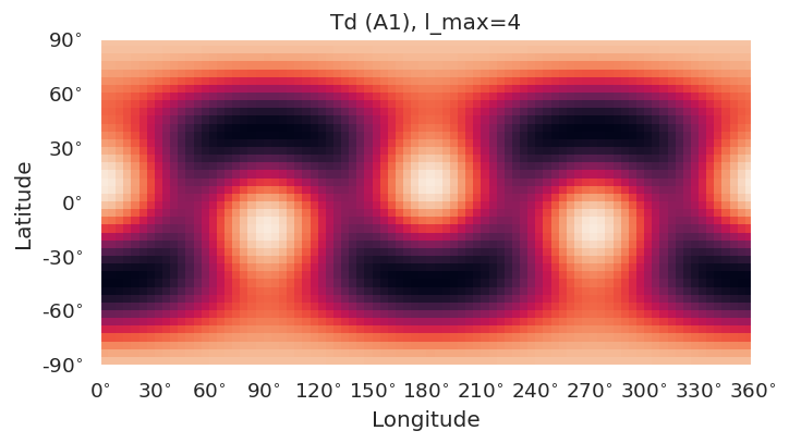
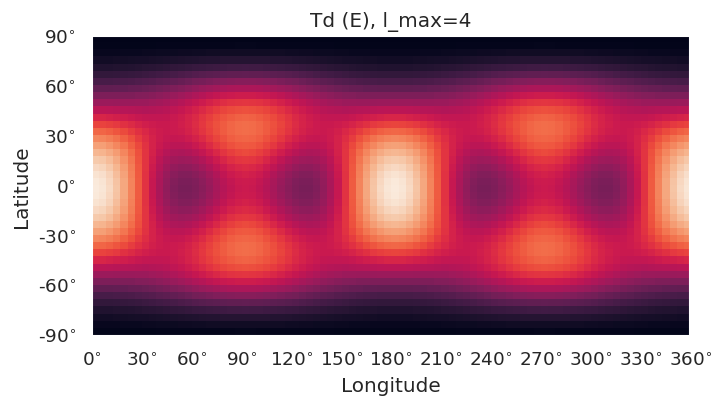
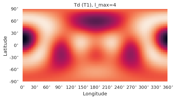
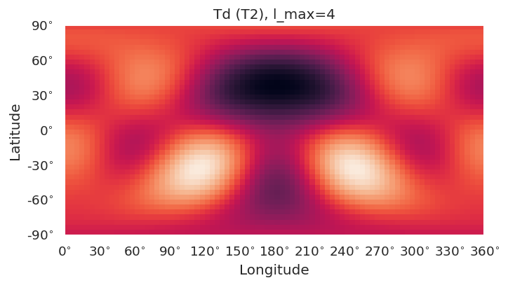
Visualisation

Basic routines are currently implemented using SHtools plotting functionality.

self.plotXlm() will plot maps for each character (all harmonics), or specified character if passed. This wraps SHtools grid.plot() method, and **kwargs are passed directly, as:

grid = self.clm[key][pType].expand(lmax = gridlmax)
grid.plot(title=f'{self.PG} ({key}), l_max={self.lmax}', **kwargs)

SHtools objects can be accessed directly via self.coeffs['SH'][char][type], and all SHtools class methods can be called. (See below.)

TODO: interface to ePSproc plotting routines and subselection.

[7]:

# Plot maps
symObj.plotXlm()

/home/femtolab/anaconda3/envs/epsdev-030821/lib/python3.7/site-packages/pyshtools/shclasses/shcoeffsgrid.py:3568: UserWarning: Matplotlib is currently using module://ipykernel.pylab.backend_inline, which is a non-GUI backend, so cannot show the figure.
  fig.show()

../_images/sym_pemtk_symHarm_demo_160322_tidy_18_1.png

../_images/sym_pemtk_symHarm_demo_160322_tidy_18_2.png

../_images/sym_pemtk_symHarm_demo_160322_tidy_18_3.png

../_images/sym_pemtk_symHarm_demo_160322_tidy_18_4.png

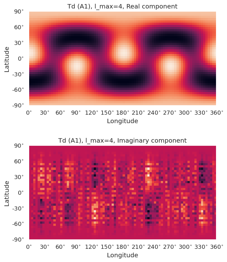
[8]:

# Plot maps for specified character and type
# Note for complex harmonics, both real and imaginary maps are shown
# Note colour bar not working for pySHtools v4.5, but OK in v4.9
symObj.plotXlm(pType = 'comp', syms=['A1'], colorbar = 'right')

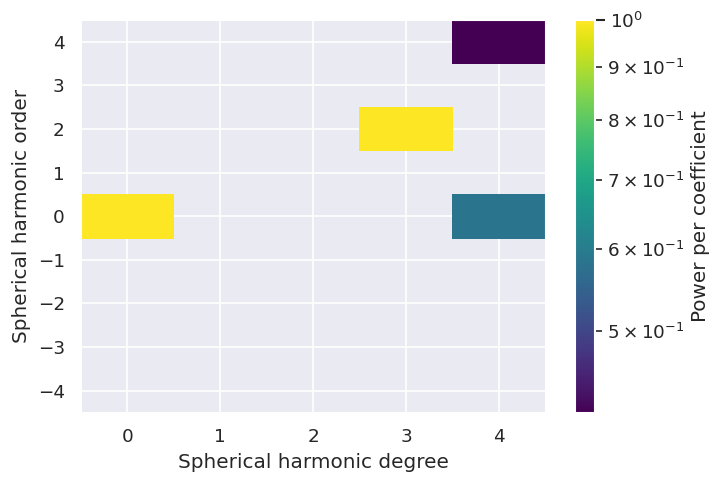
../_images/sym_pemtk_symHarm_demo_160322_tidy_19_0.png

[9]:

# Coeffs can also be visualised with the SHtools method plot_specturm2d()
symObj.coeffs['SH']['A1']['real'].plot_spectrum2d()

/home/femtolab/anaconda3/envs/epsdev-030821/lib/python3.7/site-packages/pyshtools/shclasses/shcoeffsgrid.py:2035: UserWarning: Matplotlib is currently using module://ipykernel.pylab.backend_inline, which is a non-GUI backend, so cannot show the figure.
  fig.show()

[9]:

(<Figure size 720x480 with 2 Axes>,
 <matplotlib.axes._subplots.AxesSubplot at 0x7f4a3d014110>)

../_images/sym_pemtk_symHarm_demo_160322_tidy_20_2.png

Raw data outputs

Raw data is available as Pandas DataFrames, SHtools and Xarray objects, via the self.coeffs dictionary.

[10]:

symObj.coeffs.keys()

[10]:

dict_keys(['libmsym', 'DF', 'SH', 'XR'])

[11]:

# Dataframes are nested by type
# (real coeff)
symObj.coeffs['DF']['real']

[11]:

					b (real)
C	h	mu	l	m
A1	0	0	0	0	1.000000
	1	0	3	-2	1.000000
	2	0	4	0	0.763763
	2	0	4	4	0.645497
E	0	0	2	0	0.500000
		0	2	2	0.866025
		1	2	0	-0.866025
		1	2	2	0.500000
	1	0	4	0	0.322749
				2	-0.866025
				4	-0.381881
		1	4	0	-0.559017
				2	-0.500000
				4	0.661438
T1	0	0	3	1	0.790569
		0	3	3	0.612372
		1	3	2	-1.000000
		2	3	-3	-0.612372
		2	3	-1	0.790569
	1	0	4	-3	0.353553
		0	4	-1	0.935414
		1	4	-4	-1.000000
		2	4	1	0.935414
		2	4	3	-0.353553
T2	0	0	1	1	1.000000
		1	1	0	-1.000000
		2	1	-1	1.000000
	1	0	2	-1	1.000000
		1	2	-2	-1.000000
		2	2	1	1.000000
	2	0	3	1	0.612372
		0	3	3	-0.790569
		1	3	0	1.000000
		2	3	-3	0.790569
		2	3	-1	0.612372
	3	0	4	-3	0.935414
		0	4	-1	-0.353553
		1	4	-2	-1.000000
		2	4	1	-0.353553
		2	4	3	-0.935414

[12]:

# Dataframe (comp coeff)
symObj.coeffs['DF']['comp']

[12]:

					b (complex)
C	h	mu	l	m
A1	0	0	0	0	1.000000+0.000000j
	1	0	3	2	0.707107+0.000000j
	1	0	3	-2	-0.707107+0.000000j
	2	0	4	0	0.763763+0.000000j
	2	0	4	4	0.456435+0.000000j
...	...	...	...	...	...
T2	3	1	4	-2	0.707107+0.000000j
		2	4	1	0.250000-0.000000j
				-1	-0.250000-0.000000j
				3	0.661438-0.000000j
				-3	-0.661438-0.000000j

72 rows × 1 columns

[13]:

# SHtools object are stored in dicts by character and type
symObj.coeffs['SH']['A1']['real']

[13]:

kind = 'real'
normalization = '4pi'
csphase = 1
lmax = 4
header = None

[14]:

symObj.coeffs['SH']['A1']['real']

[14]:

kind = 'real'
normalization = '4pi'
csphase = 1
lmax = 4
header = None

[15]:

# All SHtools methods can be accessed this way, e.g. coeffs
symObj.coeffs['SH']['A1']['real'].coeffs

[15]:

array([[[1.        , 0.        , 0.        , 0.        , 0.        ],
        [0.        , 0.        , 0.        , 0.        , 0.        ],
        [0.        , 0.        , 0.        , 0.        , 0.        ],
        [0.        , 0.        , 1.        , 0.        , 0.        ],
        [0.76376262, 0.        , 0.        , 0.        , 0.64549722]],

       [[0.        , 0.        , 0.        , 0.        , 0.        ],
        [0.        , 0.        , 0.        , 0.        , 0.        ],
        [0.        , 0.        , 0.        , 0.        , 0.        ],
        [0.        , 0.        , 0.        , 0.        , 0.        ],
        [0.        , 0.        , 0.        , 0.        , 0.        ]]])

Note SHTOOLS array indexing, from fortran docs: https://shtools.oca.eu/shtools/public/using-with-f95.html

$C_{lm} = \left \lbrace \begin{array}{ll} \mbox{clm}(1,l+1,m+1) & \mbox{if } m\ge 0 \\ \mbox{clm}(2,l+1,m+1) & \mbox{if } m < 0.\\ \end{array} \right.$

(For python case don’t need +1 for indexes.)

[16]:

# Xarray version - this has both real and comp types as a Dataset
symObj.coeffs['XR']

[16]:

<xarray.Dataset>
Dimensions:      (C: 4, LM: 45, inds: 12)
Coordinates:
  * C            (C) object 'A1' 'E' 'T1' 'T2'
  * inds         (inds) MultiIndex
  - h            (inds) int64 0 0 0 1 1 1 2 2 2 3 3 3
  - mu           (inds) int64 0 1 2 0 1 2 0 1 2 0 1 2
  * LM           (LM) MultiIndex
  - l            (LM) int64 0 0 0 0 0 0 0 0 0 1 1 1 ... 3 3 3 4 4 4 4 4 4 4 4 4
  - m            (LM) int64 -1 -2 -3 -4 0 1 2 3 4 -1 ... 4 -1 -2 -3 -4 0 1 2 3 4
Data variables:
    b (real)     (C, inds, LM) float64 nan nan nan nan ... nan -0.9354 nan
    b (complex)  (C, inds, LM) complex128 (nan+0j) (nan+0j) ... (nan+0j)

Comparison with literature values

Quick tests vs. Chandra 1987 - looks OK, although not totally clear if sign-convention is different/flipped?

816e2fb6d763412b9882dfc5e1b7bf4d

[17]:

# Chandra (1987) gives...
# OK
import numpy as np
print(f'Chandra l=3,m=+/-1: {np.sqrt(5)/(4)}')
print(f'Chandra l=3,m=+/-3: {np.sqrt(3)/(4)}')
# symObj.coeffDF.loc['T1','0', '0']
symObj.coeffs['DF']['comp'].loc['T1','0', '0'] # Subselect for T1, h=0, mu=0 (note different mu to Chandra formalism!)
# Note opposite signs for +/-m terms in this case.

Chandra l=3,m=+/-1: 0.5590169943749475
Chandra l=3,m=+/-3: 0.4330127018922193

[17]:

		b (complex)
l	m
3	1	-0.559017-0.000000j
	-1	0.559017+0.000000j
	3	0.433013-0.000000j
	-3	-0.433013-0.000000j

[18]:

# Chandra (1987) gives...
# OK
print(f'Chandra l=4,m=+/-1: {np.sqrt(7)/(4)}')
print(f'Chandra l=4,m=+/-3: {1/(4)}')  #*np.sqrt(2))
symObj.coeffs['DF']['comp'].loc['T1','1', '0'] # Subselect for T1, h=0, mu=0 (note different mu to Chandra formalism!)
# Note same signs for +/-m pairs in all cases for this set.

Chandra l=4,m=+/-1: 0.6614378277661477
Chandra l=4,m=+/-3: 0.25

[18]:

		b (complex)
l	m
4	3	0.250000-0.000000j
	-3	0.250000+0.000000j
	1	-0.661438-0.000000j
	-1	-0.661438+0.000000j

Not yet more carefully tested, but this quick sanity check looks OK.

Versions

[19]:

import scooby
scooby.Report(additional=['epsproc', 'pemtk', 'holoviews', 'hvplot', 'xarray', 'matplotlib', 'bokeh', 'pyshtools'])

[19]:

Thu Mar 24 12:20:09 2022 EDT
OS	Linux	CPU(s)	4	Machine	x86_64
Architecture	64bit	RAM	7.7 GB	Environment	Jupyter
Python 3.7.6 (default, Jan 8 2020, 19:59:22) [GCC 7.3.0]
epsproc	1.3.1-dev	pemtk	0.0.1	holoviews	1.12.6
hvplot	0.6.0	xarray	0.13.0	matplotlib	3.2.0
bokeh	1.4.0	pyshtools	4.5	numpy	1.18.1
scipy	1.3.1	IPython	7.13.0	scooby	0.5.5
Intel(R) Math Kernel Library Version 2019.0.4 Product Build 20190411 for Intel(R) 64 architecture applications

[20]:

# Check current Git commit for local ePSproc version
import pemtk
from pathlib import Path
!git -C {Path(pemtk.__file__).parent} branch
!git -C {Path(pemtk.__file__).parent} log --format="%H" -n 1

* master
6c603e299dcfeb05ea730f415a35a604c964d193

[21]:

# Check current remote commits
!git ls-remote --heads https://github.com/phockett/pemtk

6c603e299dcfeb05ea730f415a35a604c964d193        refs/heads/master

[ ]: